The appendix goal is detail description of analysis results dealing with possibility of external effects influence on measured displacement. The result analysis should give an answer to question if the measured displacement is locally dependent or independent to known external effects.

The goal is not to discuss global relation between measured displacement and external effects. This identified global relation is discussed in the main document and in appendix B - “Measured Results, Reproducibility and Space Dependency”. The analysis content is to eliminate or to confirm local direct influence of any analyzed external effect to the measured displacement.

The analyses are divided into different parts with respect of different hypotheses of possible interaction. The hypothesis directs adequate analysis method of possible relationship between external influence and measured displacement.

The analyses are based namely on measurement results from L2 locality. The reason is that there exist long time series of measured displacement and external effects measurements from L2 locality surroundings. There exist external effects measurement time series results from CHMI locality placed approximately 10 km from L2 locality [11]. It makes L2 locality the best locality for external influence study of all measurement localities.

Other locality measurement results were used for some analyses too.

Space dependency i.e. measured displacements dependency on the locality position is analysed in appendix B – “Measured Results, Reproducibility and Space Dependency”.

Linear dynamic system with constant parameters

The hypothesis based on idea that measured displacements are caused by response of linear dynamic system with constant parameters to some external effect signal, is studied in this section.

This hypothesis is equivalent to the most frequent physical systems.

The general linear dynamic system with time and signal value independent parameters is supposed. The hypothetical system output is measured displacements and input is external effect signal.

The spectral analysis is the main tool to study the linear dynamic system with constant parameters excited by periodic signal.

It is not possible to generate measurement device stimulation by artificial stimulus as usual in classical physical experimental methodology. It was not possible reliable shielding of all external effects as well. It is possible to use measured displacements and studied external effect signals spectral analysis to confirm or exclude the hypothesis.

All input signal frequencies of linear dynamic system has to be on output of the system. There must not be any other frequency on output, which is on the input. Only amplitude (and phase) of frequency line can be changed. But independent change of any spectral line is not possible. Close frequency lines must change similar way. This is result of system linearity and its constant parameters.

Noise is signal with unlimited number of frequencies in linear dynamic systems. The described discrete frequencies features are valid for linear system stimulated by noise too. The same is valid for system stimulated by mixture of noise and discrete frequencies signal. It means that input/output ratio of noise spectral lines close to discrete spectral line has to be close to discrete spectral line input/output ratio.

Two noise signals are only added in linear systems. Two discrete signals are added in most cases too. Only in case of two fully synchronous signals with opposite phase the signals are subtracted.

Discrete spectral line can “disappear” in linear system stimulated by mixture of discrete frequency and noise signal in case, if discrete spectral line is small with respect to noise on output. Noise signals mask discrete spectral line signal.

Opposite situation is impossible; it means that it is not possible isolate only one separate spectral line from noise by linear system.

Frequency analysis of all potential external effects signals was made and compared with frequency analysis of measured displacements to verify or refute the working hypothesis.

Measurement results from professional meteorological station CHMI [11] from locality Prague-Libuš and basic external variables measurement results from L2 locality was use as external effects signals. Distance between L2 locality and CHMI station is approximately 10km. L2 locality is placed approximately 20m above surrounding terrain.

All amplitudes are normalized with respect of 24hour spectral line amplitude in all cases. It enables to compare different physical signals without problems with conversion of physical units.

If possible signal 2years time series with 30min time step was used. Only in case of shorter measurement 1.6year time series with 30min time step was used.

All signals contain great amount of noise. It is not only measurement errors. Main amplitude of “noise” is caused by irregular signal component. The noise level close to separate spectral line was used to define weight of separate spectral line.

The weight is defined as separate spectral line to surrounded noise amplitude ratio. The weight represents credibility of separate spectral line. The greater spectral line weight the less influence of noise to the spectral line amplitude.

The weights are used for classification of compared spectral lines compliance or contradiction.

The full consistency (++) is defined as the case if two compared signals have spectral lines with exactly the same frequency and relative amplitudes are close each other, it means the amplitudes normalised to 24hour spectral line do not differ more than 33% with respect to the greater ones.

The full consistency is the situations if in two signals are no separated spectral lines of compared frequency. It means that in both signals separated spectral lines are missing and only noise was identified.

The approximate consistency (+) is defined as the case if two compared signals have spectral lines with exactly the same frequency and relative amplitudes are approximately each other, it means the amplitudes do not differ more than 50% with respect to the greater ones (-50% to +100% with respect to selected signal).

The contradiction is defined as the case the case if two compared signals have spectral lines with exactly the same frequency and relative amplitudes are different each other, it means the amplitudes differs more than 50% with respect to the greater ones (-50% to +100%.with respect to selected signal) or the frequency is not the same.

The contradiction is defined as the case if one signal contains spectral line with weight greater than 2 and second signal do not contains any separated spectral line (contains only noise).

The removable contradiction is defined as the case, if analyzed signal (input signal of the hypothetical system – named “IN” in the tables) contains spectral line with weight less than 5 and reference signal (output signal of hypothetical system) contains no spectral line greater than noise. It is based on the hypothetical possibility to hide the periodical signal by the noise of other input signal.

The opposite situation (named “OUT” in the tables) is supposed to be irremovable contradiction. It is based on the linear system feature, that it is impossible to gain periodic signal with significant spectral line from noise. It is possible to gain the spectral line only from another periodical signal.

The situation “IN” with weight grater than 5 is defined as irremovable contradiction. The reason is, that analyzed signal can not be greater than 20% of result signal in this situation and the second signal must be dominant in this case. It does not make sense to deal with this possibility.

The situations if one signal contains periodical signal with spectral line of weight less than 2 and second signal contains only noise in analyzed part of spectrum was not counted as relevant. The irrelevant situation (?) was not validated as consistency and was not validated as contradiction.

Analysis results and their evaluations of particular analyzed signals are described in the following text. Every signal is described in one separated section.

The section contains:

Full spectrum
Spectral areas details (24hour, 12hour, 8hour and 6hour)
Spectral line presence schema comparing relative amplitudes referenced to 24.000 hour spectral line of the analyzed signal
Spectral line presence schema comparing relative amplitudes referenced to peak noise amplitude in the analyzed spectral area of the analyzed signal (weight of analyzed spectral line)
Hypothetical system frequency characteristic with periodical signals ratios marked out with graphically visualized weight
Table comparing analyzed signal spectrum with measured displacements spectrum
Table comparing analyzed signal noise with measured displacements noise

The analysed signals are:

T-ext – external air temperature in L2 locality
T-int – internal air temperature in L2 locality
T-chmi - external air temperature measured by CHMI
RA-chmi – Sun radiation measured by CHMI
RA-u – Sun radiation proportional voltage in L2 locality
RA-uexp – recalculated Sun radiation in L2 locality
intRA-uexp – time integral of recalculated Sun radiation in L2 locality
P-chmi - atmospheric air pressure measured by CHMI
TD-chmi - dew point temperature calculated from CHMI measurement
WS-chmi - wind speed measured by CHMI
RH-chmi – external air relative humidity measured by CHMI
SS – simulated theoretical Sun radiation in L2 locality without building shielding effect
SSS – simulated theoretical Sun radiation in L2 locality with building shielding effect
L2-NS is north-south component of measured displacements in L2 locality.
L2-EW is east-west component of measured displacements in L2 locality.

T-ext

T-ext is external air temperature in free space measured in area close to external building skin (approx. 5 cm). The measurement point is very close to L2 locality (approx. 1m). It is separated from measurement device by building wall made of ferroconcrete. The Sun radiation protection of temperature sensor is simple. Secondary effect of indirect heating from building wall is very probable.

T-ext was digitally measured 3times per minute and average value with deviation was recorded onetime per minute.

The spectrum was counted from 30min averages time line in range from January 2001 to December 2002 i.e. from 35040 samples.

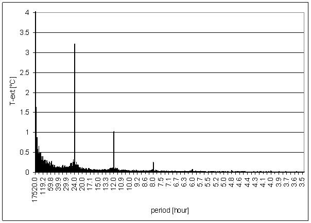
Figure 1 - T-ext full spectrum

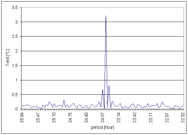
Figure 2 – 24 hour area of T-ext spectrum

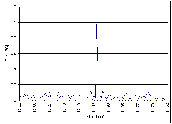
Figure 3 – 12 hour area of T-ext spectrum

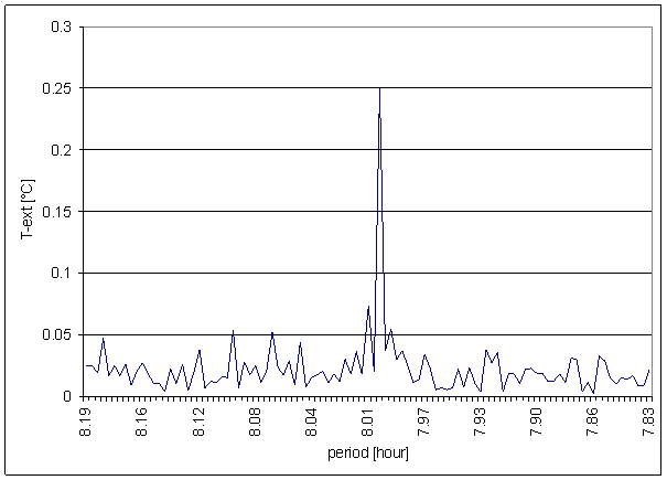
Figure 4 – 8 hour area of T-ext spectrum

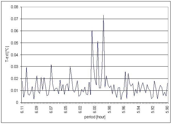
Figure 5 – 6 hour area of T-ext spectrum

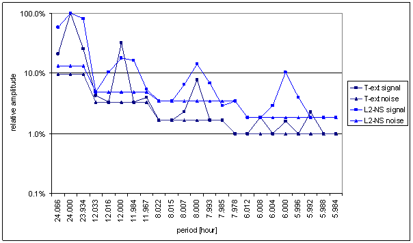
Figure 6 – Relative amplitude spectral schema of T-ext compared with L2-NS

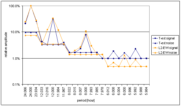
Figure 7 – Relative amplitude spectral schema of T-ext compared with L2-EW

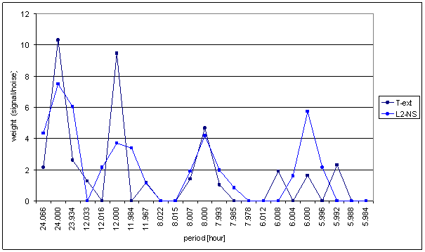
Figure 8 – Weight spectral schema of T-ext compared with L2-NS

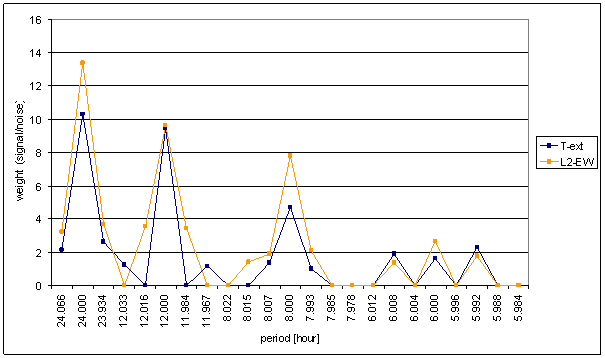
Figure 9 – Weight spectral schema of T-ext compared with L2-EW

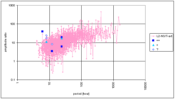
Figure 10 – Frequency characteristic of T-ext -> L2-NS hypothetical system

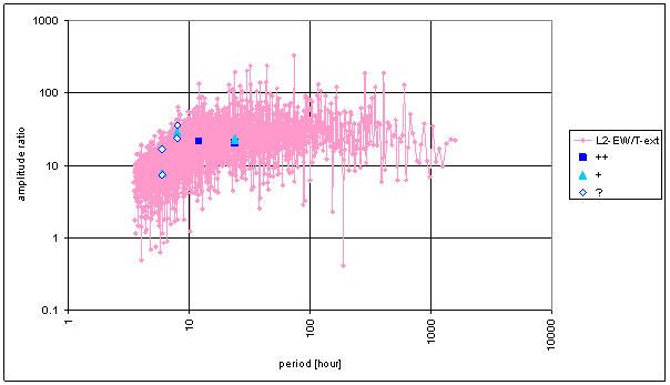
Figure 11 – Frequency characteristic of T-ext -> L2-EW hypothetical system

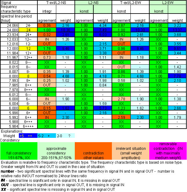
Table 1 – Correspondence evaluation of T-ext with L2-NS and L2-EW

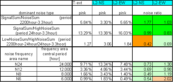
Table 2 – T-ext noise evaluation

Relatively good correspondence between T-ext and L2-EW spectrums is result of the analysis. It is the best correspondence from all directly measured external signals.

The correspondence has “small” mistakes. The deviations are visible namely in weight spectral schema, in frequency characteristics and in agreement evaluation table.

Spectral lines 12- and 12+ of T-ext are not present in L2-EW signal and spectral lines 12-- and 12++ of L2-EW are not present in T-ext signal. Similar situation is in 6hour area. Spectral lines 6- and 6+ are only in T-ext signal and 6-- and 6++ are only in L2-EW signal.

Agreement between T-ext and L2-NS is much worse.

Result of signal/noise evaluation is: T-ext can cause of L2-NS and L2-EW measured displacements.

T-int

T-int is internal temperature in the measurement device room in L2 locality measured in small distance from measurement device (approx. 0.5m). Measurement device is placed in room without window and with full door. Direct sunshine to measurement device and T-int sensor was eliminated.

T-int was digitally measured 3times per minute and average value with deviation was recorded onetime per minute.

The spectrum was counted from 30min averages time line in range from September 2001 to March 2003 i.e. from 28320 samples.

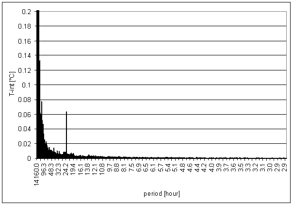
Figure 12 - T-int full spectrum

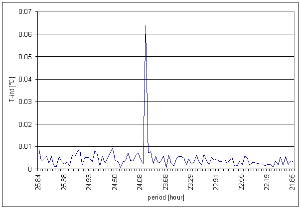
Figure 13 – 24 hour area of T-int spectrum

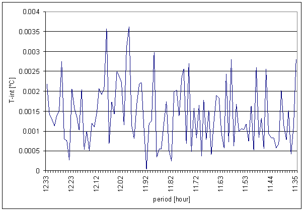
Figure 14 – 12 hour area of T-int spectrum

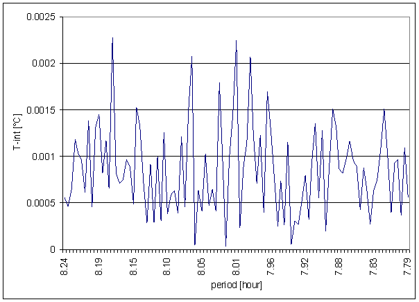
Figure 15 – 8 hour area of T-int spectrum

Figure 16 – 6 hour area of T-int spectrum

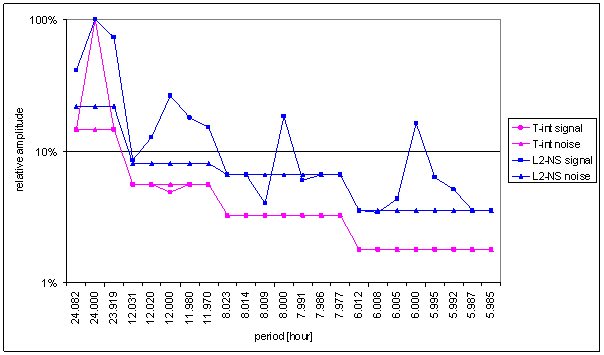
Figure 17 – Relative amplitude spectral schema of T-int compared with L2-NS

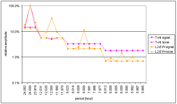
Figure 18 – Relative amplitude spectral schema of T-int compared with L2-EW

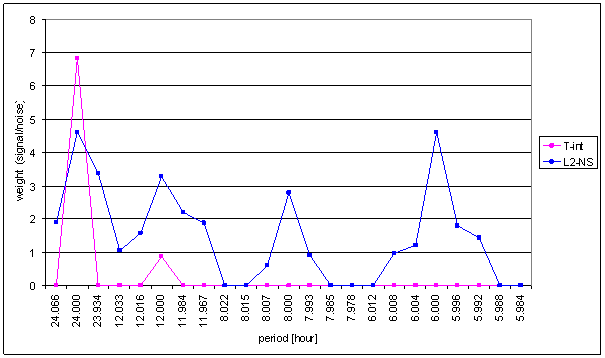
Figure 19 – Weight spectral schema of T-int compared with L2-NS

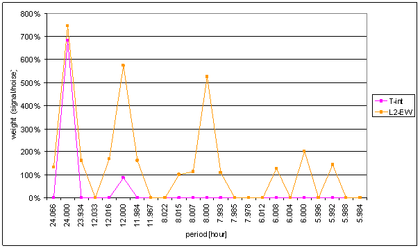
Figure 20 – Weight spectral schema of T-int compared with L2-EW

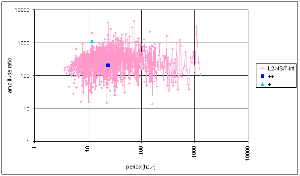
Figure 21 – Frequency characteristic of T-int -> L2-NS hypothetical system

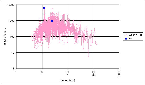
Figure 22 – Frequency characteristic of T-int -> L2-EW hypothetical system

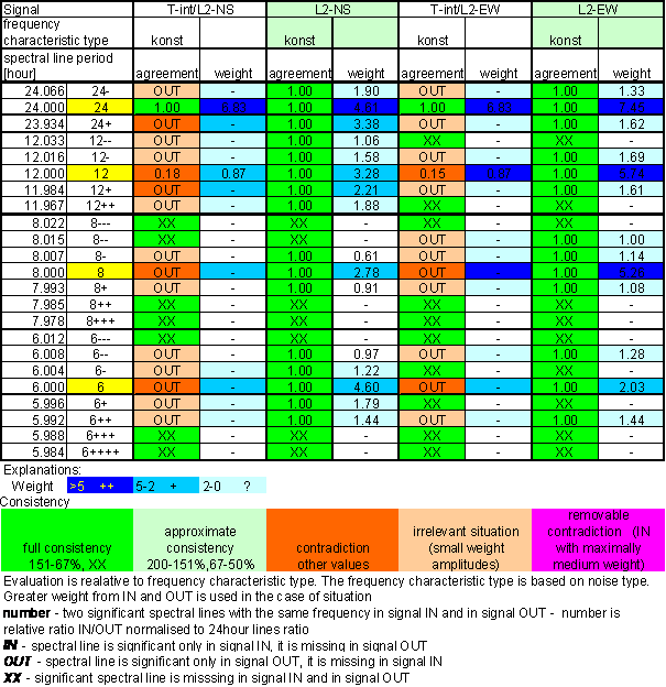
Table 3 – Correspondence evaluation of T-int with L2-NS and L2-EW

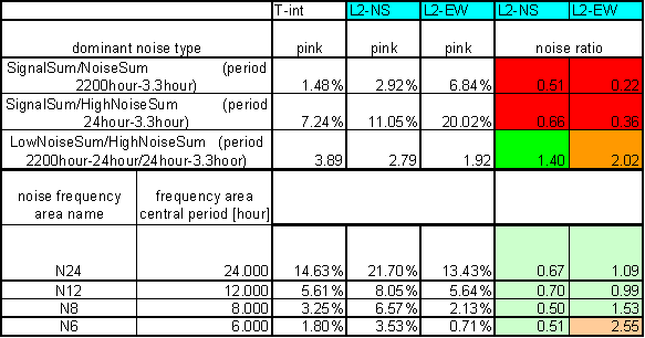
Table 4 – T-int noise evaluation

Great difference between T-int and measured displacements spectrums is result of the analysis. It is the worst correspondence from all external signals.

Result of signal/noise evaluation is: T-int can not be cause of L2-NS or L2-EW measured displacements.

T-chmi

T-chmi is standard air temperature. T-chmi was measured by professional meteorological institute CHMI in Prague-Libuš locality by MILOS measurement system. The CHMI locality is about 10 km distant from L2 locality.

Measurement results have 30min time step.

The spectrum was counted from 30min averages time line in range January 2001 to December 2002 i.e. from 35040 samples.

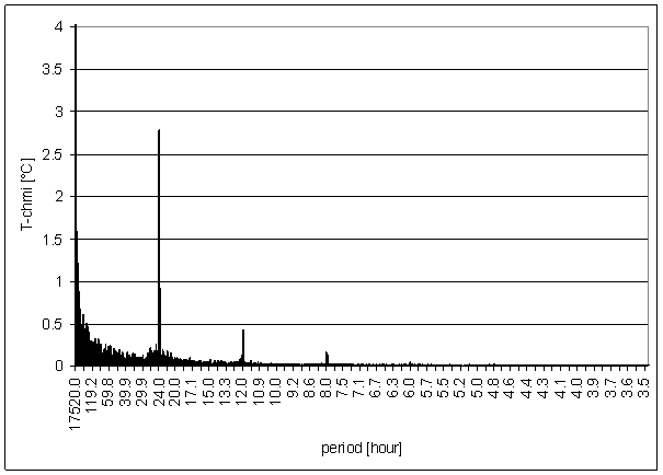
Figure 23 - T-chmi full spectrum

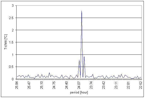
Figure 24 – 24 hour area of T-chmi spectrum

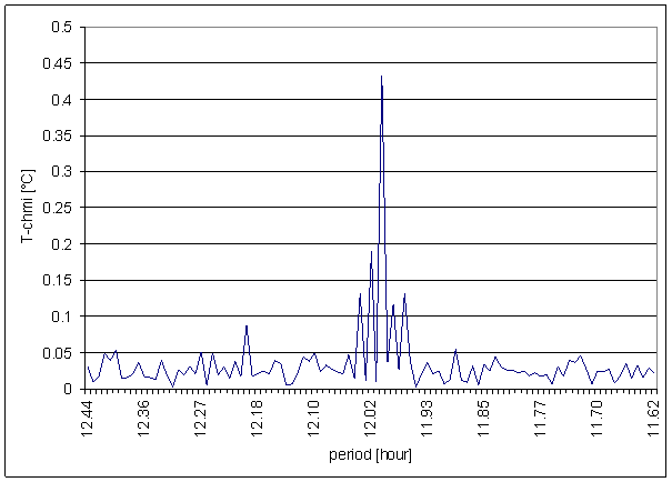
Figure 25 – 12 hour area of T-chmi spectrum

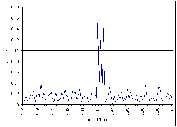
Figure 26 – 8 hour area of T-chmi spectrum

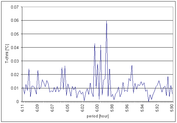
Figure 27 – 6 hour area of T-chmi spectrum

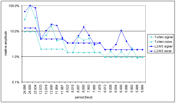
Figure 28 – Relative amplitude spectral schema of T-chmi compared with L2-NS

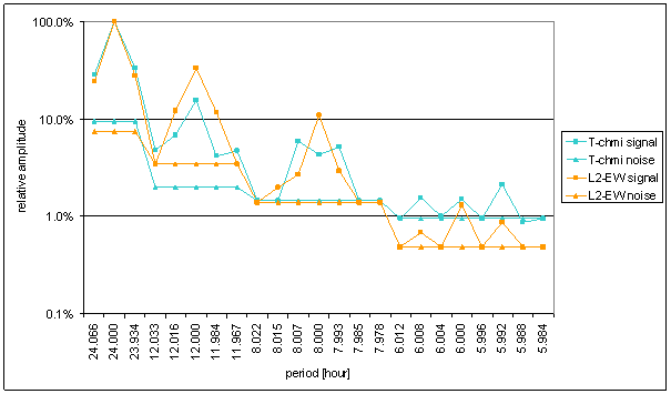
Figure 29 – Relative amplitude spectral schema of T-chmi compared with L2-EW

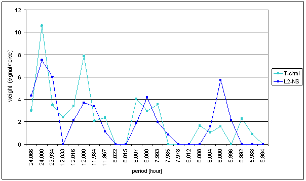
Figure 30 – Weight spectral schema of T-chmi compared with L2-NS

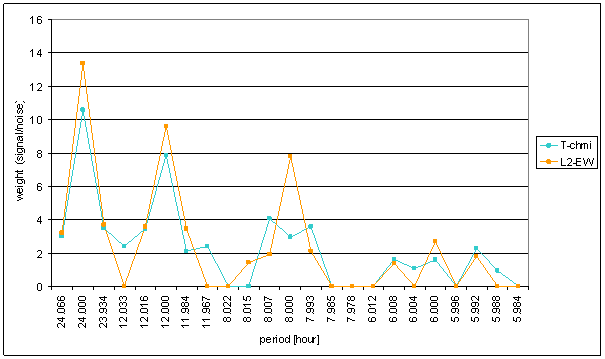
Figure 31 – Weight spectral schema of T-chmi compared with L2-EW

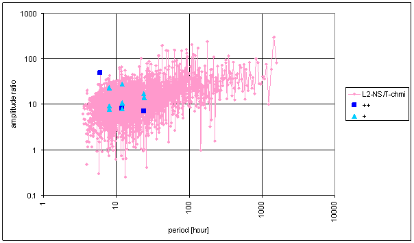
Figure 32 – Frequency characteristic of T-chmi -> L2-NS hypothetical system

Figure 33 – Frequency characteristic of T-chmi -> L2-EW hypothetical system

Table 5 – Correspondence evaluation of T-chmi with L2-NS and L2-EW

Table 6 – T-chmi noise evaluation

Medium correspondence between T-chmi and the measured displacements spectrums is result of the analysis. Some external signals have better correspondence level and other ones have worse correspondence level.

Principal contradictions (with great weight) are spectral lines 12 and 8 of L2-EW and spectral line 6 of L2-NS. Other contradictions with medium weight were identified.

Result of signal/noise evaluation is: T-chmi can be cause of L2-NS and L2-EW measured displacements.

RA-chmi

RA-chmi is radiation of the Sun. RA-chmi was measured by professional meteorological institute CHMI in Prague-Libuš locality by MILOS measurement system.

Measurement results have 30min time step.

The spectrum was counted from 30min averages time line in range January 2001 to December 2002 i.e. from 35040 samples.

Figure 34 - RA-chmi full spectrum

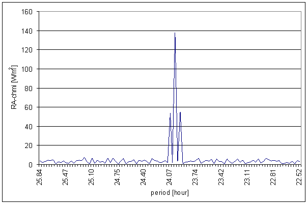
Figure 35 – 24 hour area of RA-chmi spectrum

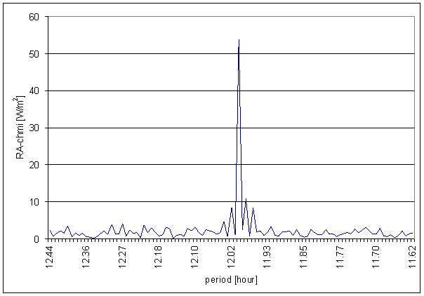
Figure 36 – 12 hour area of RA-chmi spectrum

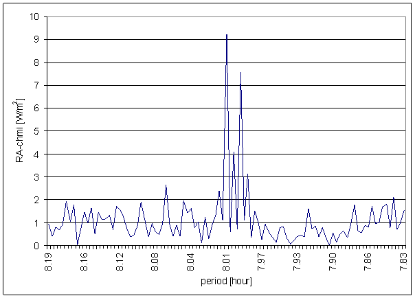
Figure 37 – 8 hour area of RA-chmi spectrum

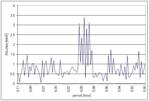
Figure 38 – 6 hour area of RA-chmi spectrum

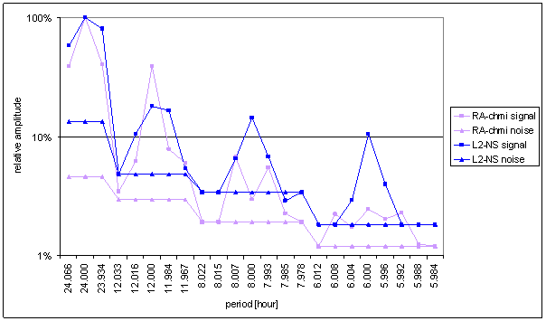
Figure 39 – Relative amplitude spectral schema of RA-chmi compared with L2-NS

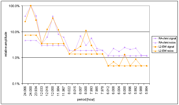
Figure 40 – Relative amplitude spectral schema of RA-chmi compared with L2-EW

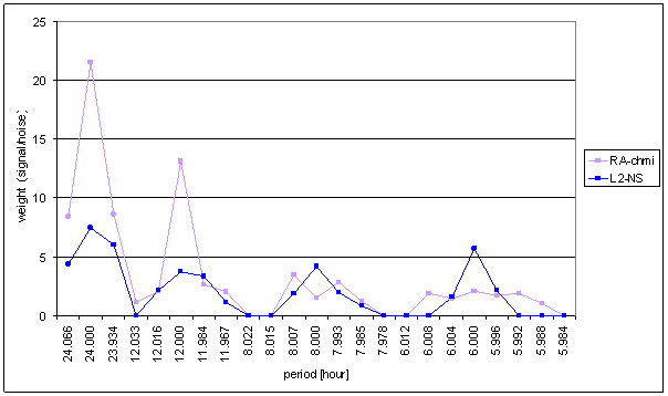
Figure 41 – Weight spectral schema of RA-chmi compared with L2-NS

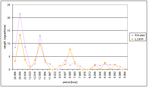
Figure 42 – Weight spectral schema of RA-chmi compared with L2-EW

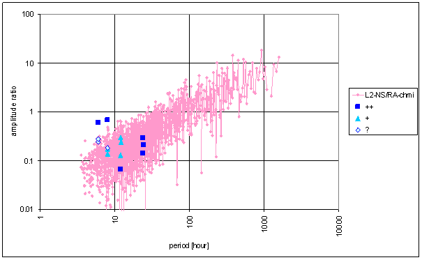
Figure 43 – Frequency characteristic of RA-chmi -> L2-NS hypothetical system

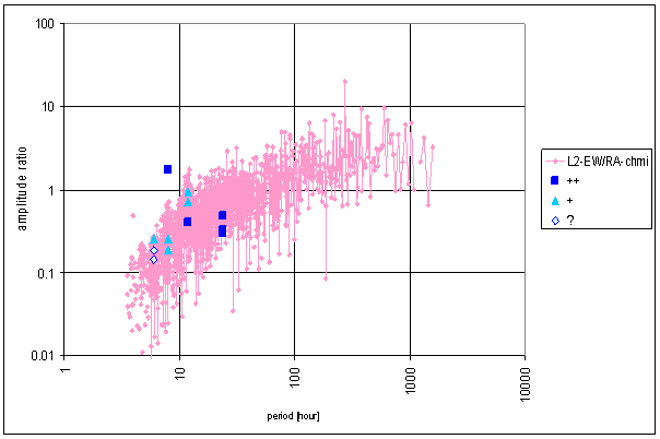
Figure 44 – Frequency characteristic of RA-chmi -> L2-EW hypothetical system

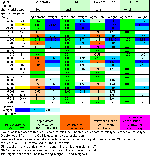
Table 7 – Correspondence evaluation of RA-chmi with L2-NS and L2-EW

Table 8 – RA-chmi noise evaluation

Medium correspondence between RA-chmi and the measured displacements spectrums is result of the analysis. Some external signals have better correspondence level and other ones have worse correspondence level.

Integrating frequency characteristics for correspondence evaluation had to be used. It reflexes noise comparison.

Principal contradictions (with great weight) are spectral line 8 of L2-EW and spectral lines 8 and 6 of L2-NS. Other contradictions with medium weight were identified.

Results of signal/noise evaluation are:

RA-chmi noise is another type than measured displacement noise (white – pink)
Digital integration of RA-chmi signal changed noise type to pink noise
Integrated RA-chmi can cause L2-NS measured displacements
Integrated RA-chmi probably can cause L2-EW measured displacements

RA-u

RA-u is output voltage of simple light intensity sensor. The sensor is placed close to external building skin (approx. 5 cm). The measurement point is very close to L2 locality (approx. 1m).

The sensor output voltage is proportional to logarithm of sensor photodiode current. Photodiode spectral characteristics and light intensity/current transfer function are not guaranteed.

The sensor has external temperature dependency of logarithmic converter. The converter temperature is close to measured external temperature T-ext.

RA-u is signal approximately proportional to logarithm of the Sun radiation in L2 locality.

RA-u was digitally measured 3times per minute and average value and deviation was recorded onetime per minute.

The spectrum was counted from 30min averages time line in range September 2001 to March 2003 i.e. from 28320 samples.

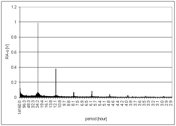
Figure 45 - RA-u full spectrum

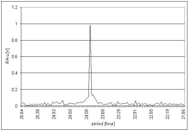
Figure 46 – 24 hour area of RA-u spectrum

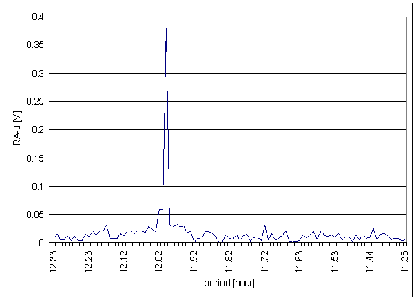
Figure 47 – 12 hour area of RA-u spectrum

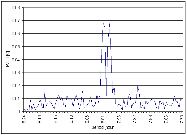
Figure 48 – 8 hour area of RA-u spectrum

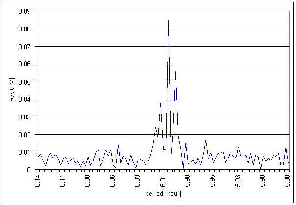
Figure 49 – 6 hour area of RA-u spectrum

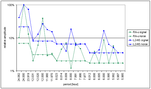
Figure 50 – Relative amplitude spectral schema of RA-u compared with L2-NS

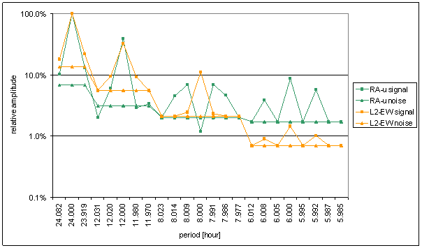
Figure 51 – Relative amplitude spectral schema of RA-u compared with L2-EW

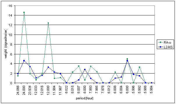
Figure 52 – Weight spectral schema of RA-u compared with L2-NS

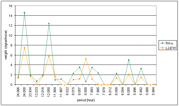
Figure 53 – Weight spectral schema of RA-u compared with L2-EW

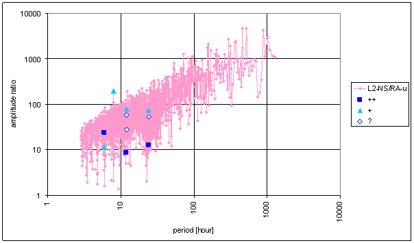
Figure 54 – Frequency characteristic of RA-u -> L2-NS hypothetical system

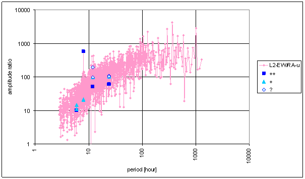
Figure 55 – Frequency characteristic of RA-u -> L2-EW hypothetical system

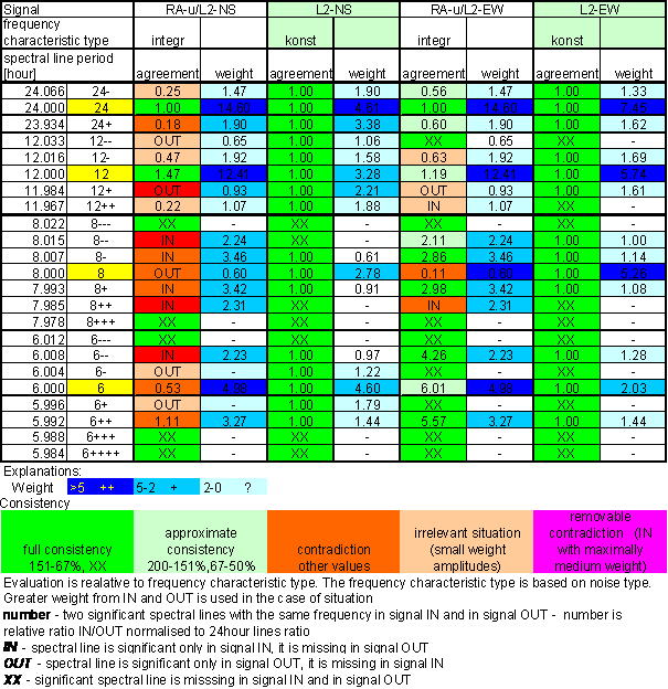
Table 9 – Correspondence evaluation of RA-u with L2-NS and L2-EW

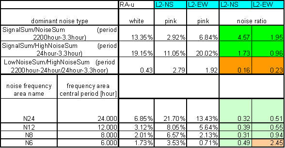
Table 10 – RA-u noise evaluation

Worse correspondence between RA-u and the L2-NS measured displacement spectrums with respect of RA-chmi is result of the analysis. Better correspondence between RA-u and the L2-EW measured displacements spectrums with respect of RA-chmi is result of the analysis too. The correspondence level of L2-EW is close to T-ext correspondence.

RA-u has medium difference in 8hour spectral area and small contradiction in 12 hour area but T-ext has medium contradictions in 12hour and 6hour areas.

Integrating frequency characteristics for correspondence evaluation had to be used. It reflexes noise comparison.

Results of signal/noise evaluation are:

RA-u noise has another type than measured displacement noise (white – pink)
Digital integration of RA-u signal changed noise type to pink noise
Integrated RA-u can be cause of L2-NS and L2-EW measured displacements

The noise area in hypothetical system frequency characteristic is sharply limited and relatively narrow, namely RA-u à L2-EW. It is contrast with the great influence of other errors to RA-u caused by simple sensor construction (namely external temperature).

RA-uexp

RA-uexp should be similar to the Sun radiation in L2 locality. RA-uexp is artificial signal. RA-uexp is recalculation result of RA-u and T-ext.

RA-uexp calculation respects logarithmic transfer function of RA-u sensor and temperature dependency of the logarithmic element.

RA-uexp calculation parameters are:

Reference voltage U₀

Temperature coefficient of reference voltage KtU₀
Logarithm reference parameter K₀
Temperature coefficient of logarithm reference parameter KtK₀

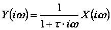
RA-uexp equation (1) is:

(1)

Transformation parameters were selected to get the best global correspondence between RA-uexp and RA-chmi in whole common measured time interval.

The spectrum was counted from calculated signal RA-uexp 30min time samples in range September 2001 to March 2003 i.e. from 28320 samples. The RA-uexp was counted from RA-u and T-ext 30min averages time lines.

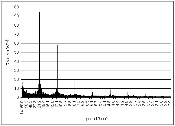
Figure 56 - RA-uexp full spectrum

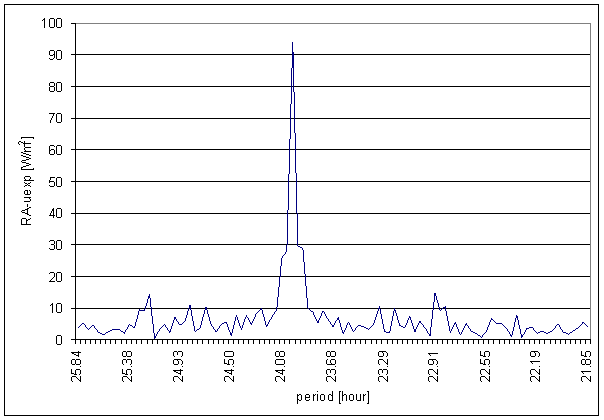
Figure 57 – 24 hour area of RA-uexp spectrum

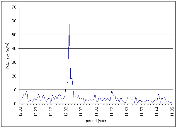
Figure 58 – 12 hour area of RA-uexp spectrum

Figure 59 – 8 hour area of RA-uexp spectrum

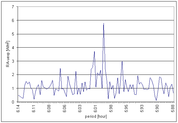
Figure 60 – 8 hour area of RA-uexp spectrum

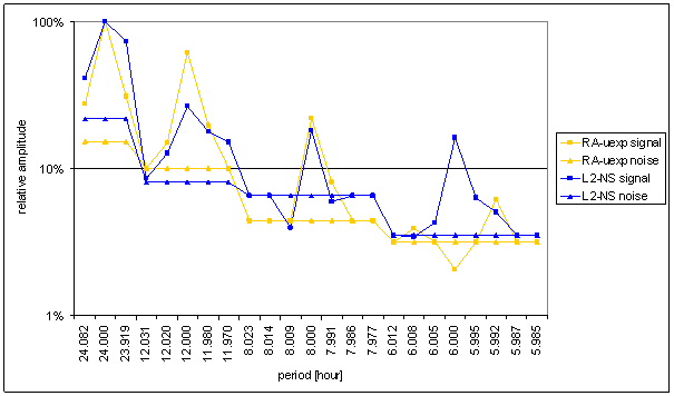
Figure 61 – Relative amplitude spectral schema of RA-uexp compared with L2-NS

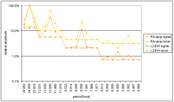
Figure 62 – Relative amplitude spectral schema of RA-uexp compared with L2-EW

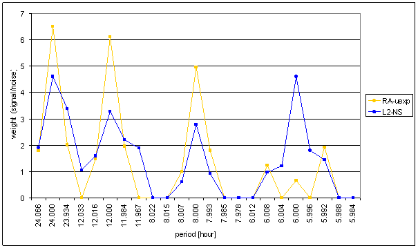
Figure 63 – Weight spectral schema of RA-uexp compared with L2-NS

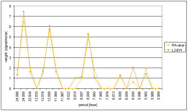
Figure 64 – Weight spectral schema of RA-uexp compared with L2-EW

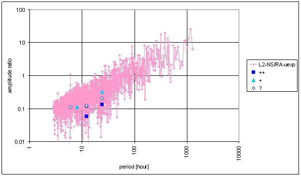
Figure 65 – Frequency characteristic of RA-uexp -> L2-NS hypothetical system

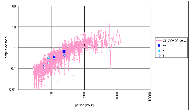
Figure 66 – Frequency characteristic of RA-uexp -> L2-EW hypothetical system

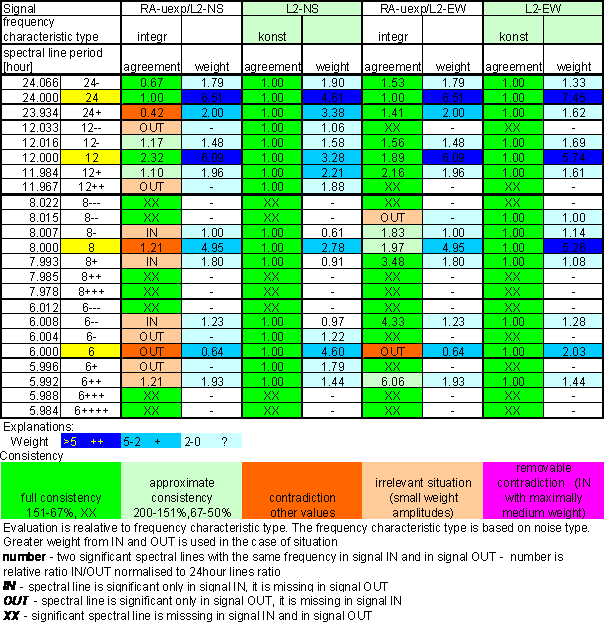
Table 11 – Correspondence evaluation of RA-uexp with L2-NS and L2-EW

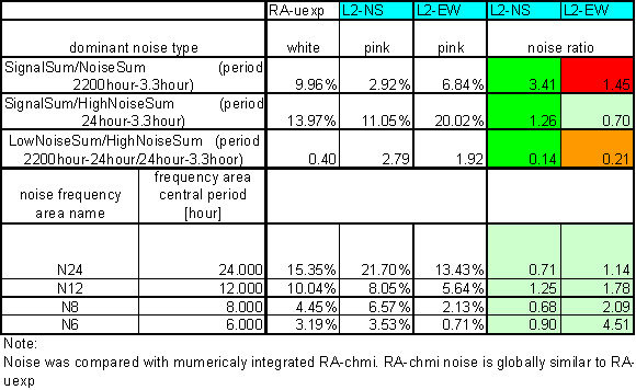
Table 12 – RA-uexp noise evaluation

Relative good correspondence between RA-u and the L2-EW measured displacement spectrums is result of the analysis.

RA-uexp signal spectrum has better correspondence with L2-EW than T-ext (and RA-u). The only medium contradiction is missing spectral line 6 in the RA-uexp signal. The weight of spectral line 6 in L2-EW is only 2.03. It is on the edge of irrelevant situation.

Correspondence between RA-uexp and L2-NS is much worse. It is better than RA-u to L2-NS correspondence.

Integrating frequency characteristics for correspondence evaluation had to be used. It reflexes noise comparison.

Result of signal/noise evaluation is the same as in case of RA-chmi (digitally integrated RA-chmi signal was used for evaluation).

The noise area in hypothetical system frequency characteristic is sharply limited and relatively very narrow, namely RA-uexp à L2-EW. The situation is more noticeable than in RA-u case.

Hypothetical system frequency characteristics implicates the idea, that integrating system with time constant value approximately 100hour (5day) can give better approximation of L2-EW.

intRA-uexp

intRA-uexp is numerically integrated signal RA-uexp. Pure time integration is defined by equation (2).

(2)

The result of the pure integration of radiation (nonnegative function) is monotony non-decreasing function. It has no physical sense.

Digital filter with transfer function (3) was used.

(3)

Time constant t defines frequency characteristic breakage. Angle speed w is 2pf where f is frequency.

Parameter t value was unknown. Several t values were defined and results were analyzed.

Basic value t=120hour was defined. Additional values t=24hour and t=600hour were defined to test result sensitivity on t value.

The spectrum was counted from numerically integrated signal intRA-uexp 30min time samples in range from September 2001 to March 2003 i.e. from 28320 samples. The intRA-uexp was counted from RA-uexp 30min time samples by digital filter.

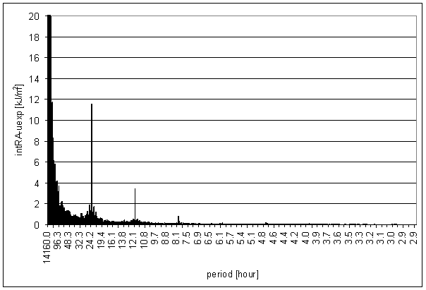
Figure 67 - intRA-uexp t=120hour full spectrum

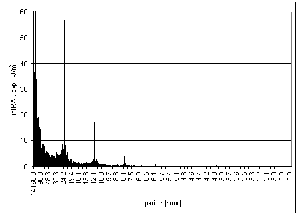
Figure 68 - intRA-uexp t=24hour full spectrum

Figure 69 - intRA-uexp t=600hour full spectrum

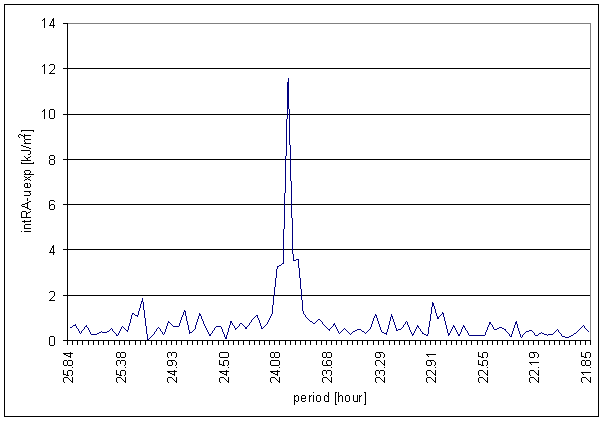
Figure 70 – 24 hour area of intRA-uexp t=120hour spectrum

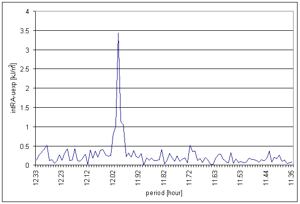
Figure 71 – 12 hour area of intRA-uexp t=120hour spectrum

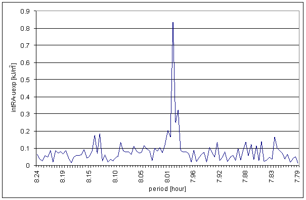
Figure 72 – 8 hour area of intRA-uexp t=120hour spectrum

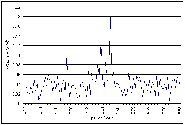
Figure 73 – 6 hour area of intRA-uexp t=120hour spectrum. The intRA-uexp spectrums are very similar to displayed spectrum for different time constant values t=24hour and t=600hour.

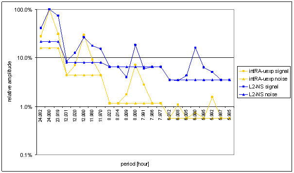
Figure 74 – Relative amplitude spectral schema of intRA-uexp t=120hour compared with L2-NS

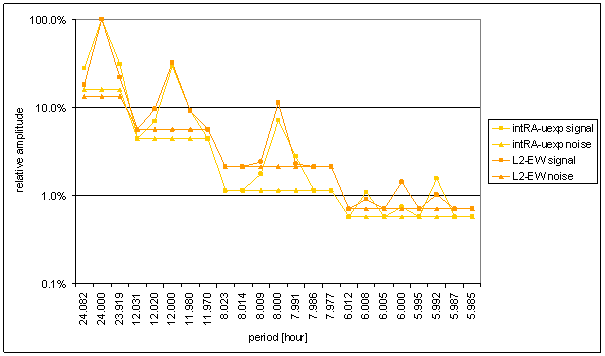
Figure 75 – Relative amplitude spectral schema of intRA-uexp t=120hour compared with L2-EW

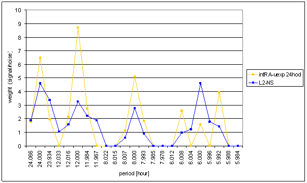
Figure 76 – Weight spectral schema compared of RA-uexp t=120hour with L2-NS

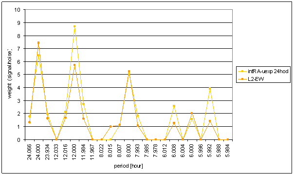
Figure 77 – Weight spectral schema of RA-uexp t=120hour compared with L2-EW. The intRA-uexp schemas are very similar to displayed schemas for different time constant values t=24hour and t=600hour.

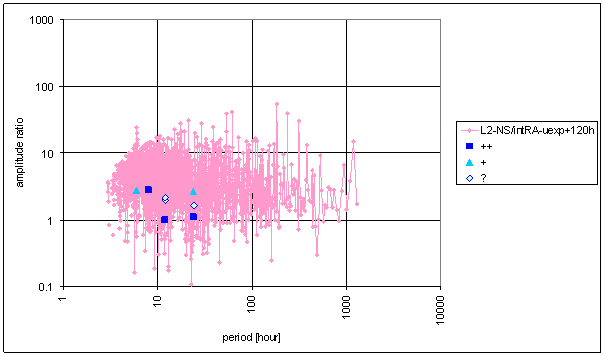
Figure 78 – Frequency characteristic of intRA-uexp t=120hour -> L2-NS hypothetical system

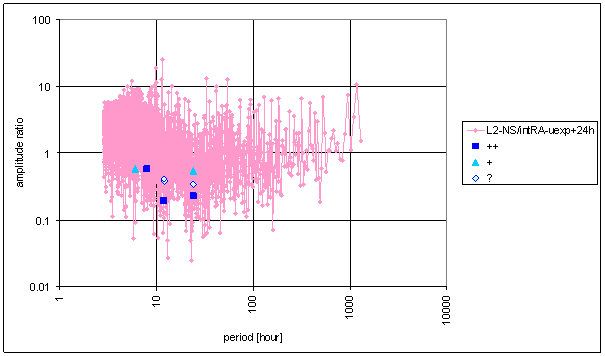
Figure 79 – Frequency characteristic of intRA-uexp t=24hour -> L2-NS hypothetical system

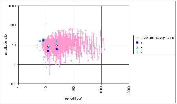
Figure 80 – Frequency characteristic of intRA-uexp t=600hour -> L2-NS hypothetical system

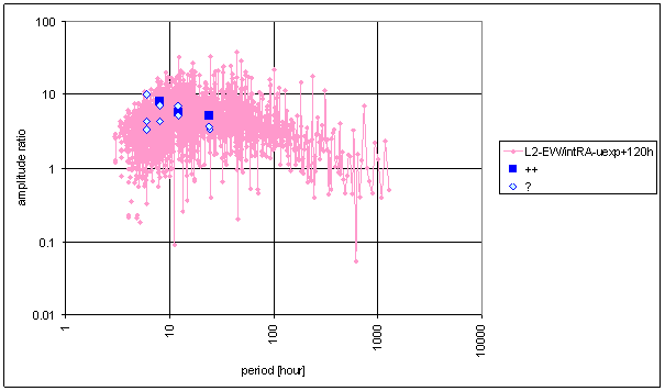
Figure 81 – Frequency characteristic of intRA-uexp t=120hour -> L2-EW hypothetical system

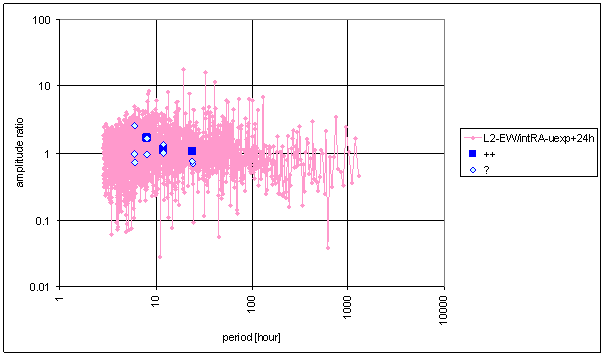
Figure 82 – Frequency characteristic of intRA-uexp t=24hour -> L2-EW hypothetical system

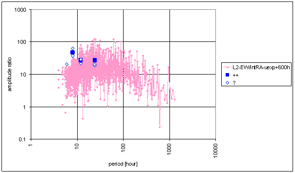
Figure 83 – Frequency characteristic of intRA-uexp t=600hour -> L2-EW hypothetical system

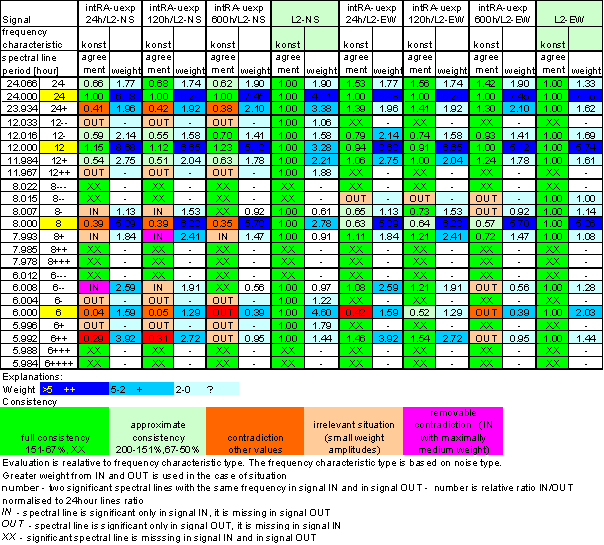
Table 13 – Correspondence evaluation of intRA-uexp with L2-NS and L2-EW

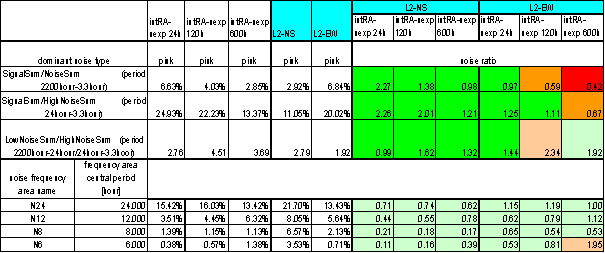
Table 14 – intRA-uexp noise evaluation

Good correspondence between intRA-uexp and the L2-EW measured displacement spectrums is result of the analysis. It is valid for both relative amplitude comparison and weight comparison i.e. amplitude/noise ratio comparison. The best correspondence is for time constant value t=120hour. Other values give little bit worse correspondence.

Spectrum correspondence intRA-uexp and L2-EW is the best correspondence from all analyzed signals.

Noise evaluation results show the clear dependency of noise parameters on time constant t value. Great value of time constant t brings great amount of low frequency noise. It decreases signal/noise ratios. Low values of time constant t (comparable with periodic signal period – 24 hours) changes periodic signal spectral line relations and destroys spectrum correspondence.

The best straightened noise frequency characteristics gives numeric filter using time constant value t=24hour.

The noise area in hypothetical system frequency characteristic is not sharply limited and is not relatively narrow, as in the case RA-uexp.

With respects of these notes, the intRA-uexp frequency characteristic is the closest to the L2-EW one.

Correspondence between RA-uexp and L2-NS is much worse. There is not good correspondence of frequency characteristics and noise parameters.

P-chmi

P-chmi is standard atmospheric pressure. P-chmi was measured by professional meteorological institute CHMI in Prague-Libuš locality by MILOS measurement system.

Measurement results have 30min time step.

The spectrum was counted from 30min averages time line in range from January 2001 to December 2002 i.e. from 35040 samples.

The spectrum was calculated from relative pressure to minimize unit pulse effect in spectrum. Relative pressure was difference of real pressure from value 1000hPa.

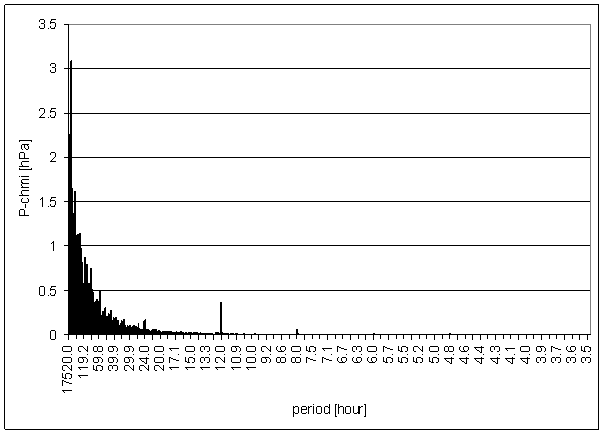
Figure 84 - P-chmi full spectrum

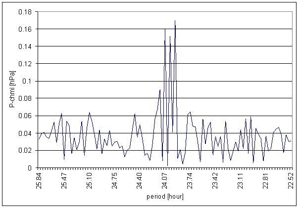
Figure 85 – 24 hour area of P-chmi spectrum

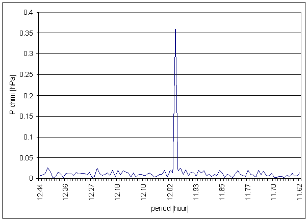
Figure 86 – 12 hour area of P-chmi spectrum

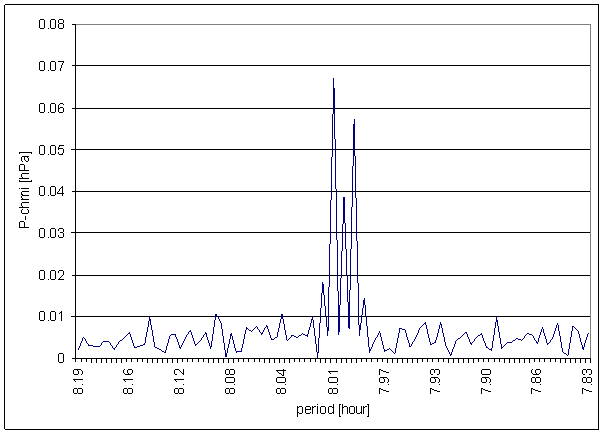
Figure 87 – 8 hour area of P-chmi spectrum

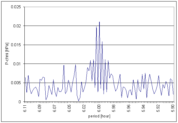
Figure 88 – 6 hour area of P-chmi spectrum

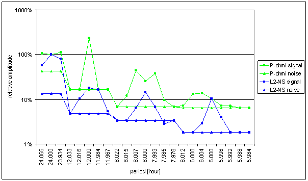
Figure 89 – Relative amplitude spectral schema of P-chmi compared with L2-NS

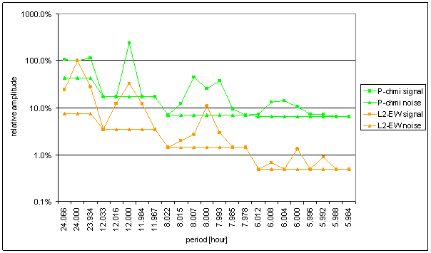
Figure 90 – Relative amplitude spectral schema of P-chmi compared with L2-EW

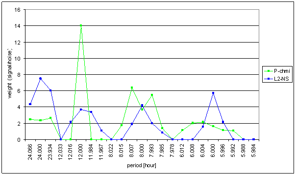
Figure 91 – Weight spectral schema of P-chmi compared with L2-NS

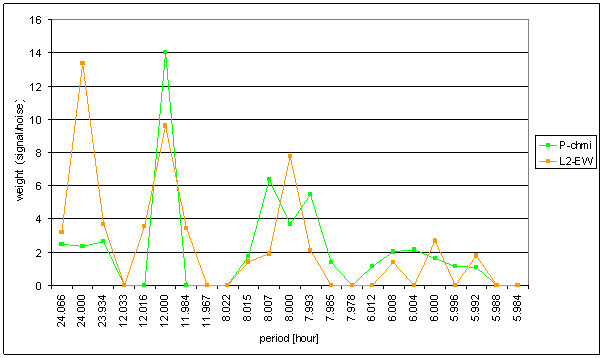
Figure 92 – Weight spectral schema of P-chmi compared with L2-EW

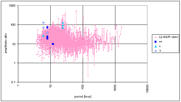
Figure 93 – Frequency characteristic of P-chmi -> L2-NS hypothetical system

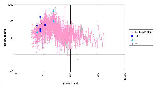
Figure 94 – Frequency characteristic of P-chmi -> L2-EW hypothetical system

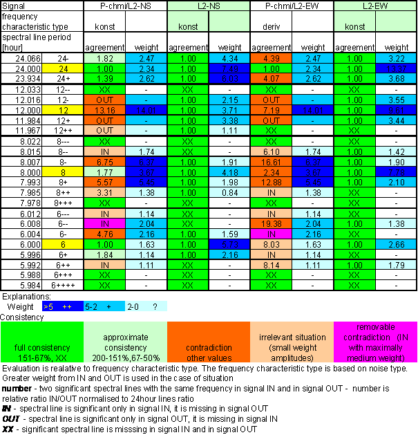
Table 15 – Correspondence evaluation of P-chmi with L2-NS and L2-EW

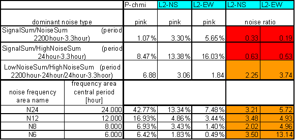
Table 16 – P-chmi noise evaluation

The great contradiction between P-chmi and measured displacements spectrums is result of the analysis.

Result of signal/noise evaluation is: P-chmi can not cause L2-NS or L2-EW measured displacements.

TD-chmi

TD-chmi is dew point temperature. TD-chmi was calculated from external temperature and relative humidity by professional meteorological institute CHMI in Prague-Libuš locality by MILOS measurement system.

Measurement results have 30min time step.

The spectrum was counted from 30min averages time line in range from January 2001 to December 2002 i.e. from 35040 samples.

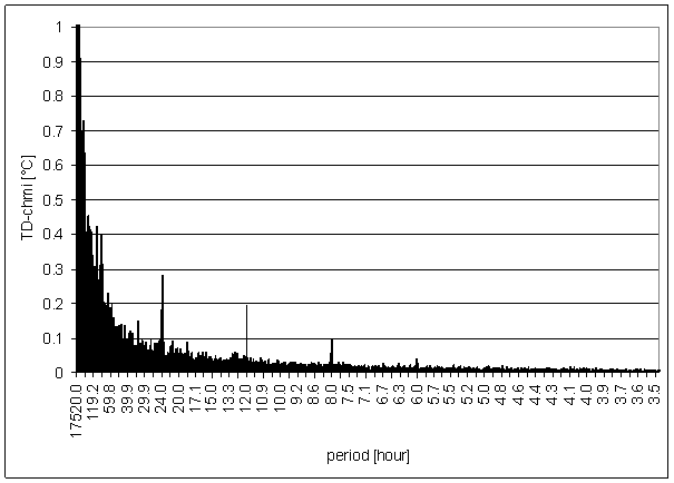
Figure 95 - TD-chmi full spectrum

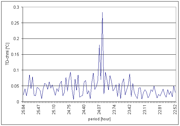
Figure 96 – 24 hour area of TD-chmi spectrum

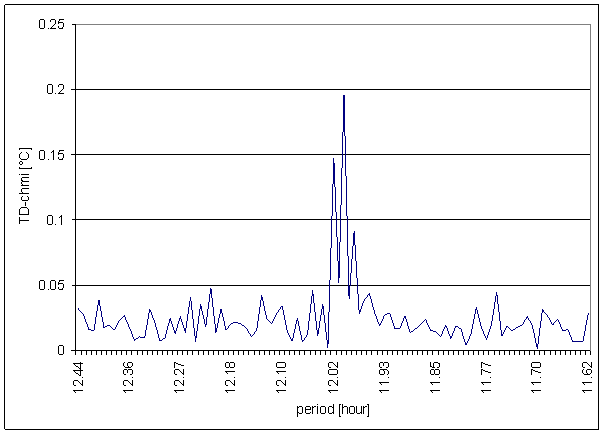
Figure 97 – 12 hour area of TD-chmi spectrum

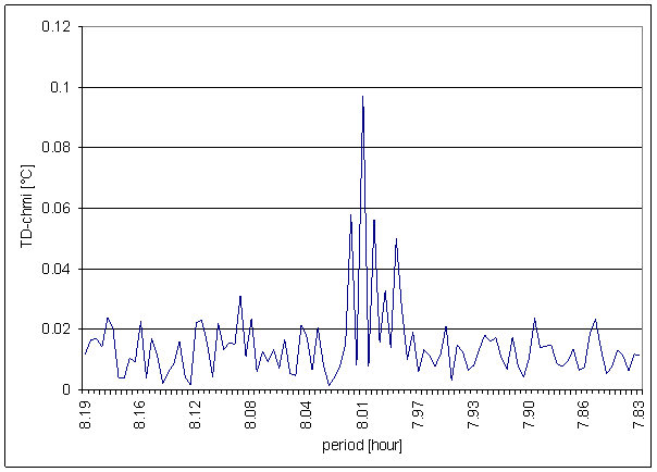
Figure 98 – 8 hour area of TD-chmi spectrum

Figure 99 – 6 hour area of TD-chmi spectrum

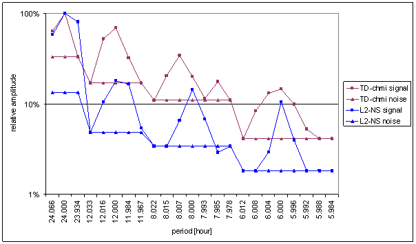
Figure 100 – Relative amplitude spectral schema of TD-chmi compared with L2-NS

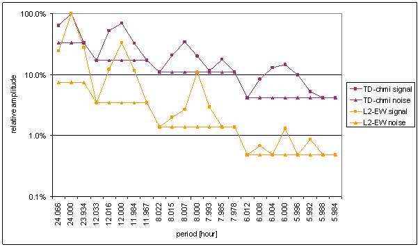
Figure 101 – Relative amplitude spectral schema of TD-chmi compared with L2-EW

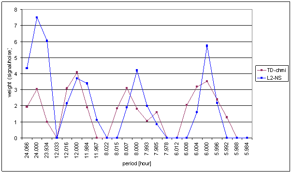
Figure 102 – Weight spectral schema of TD-chmi compared with L2-NS

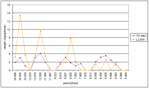
Figure 103 – Weight spectral schema of TD-chmi compared with L2-EW

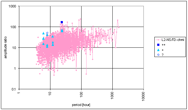
Figure 104 – Frequency characteristic of TD-chmi -> L2-NS hypothetical system

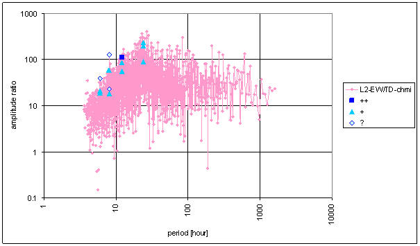
Figure 105 – Frequency characteristic of TD-chmi -> L2-EW hypothetical system

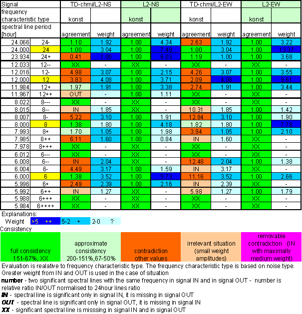
Table 17 – Correspondence evaluation of TD-chmi with L2-NS and L2-EW

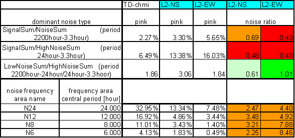
Table 18 – TD-chmi noise evaluation

The great contradiction between TD-chmi and measured displacements spectrums is result of the analysis.

Result of signal/noise evaluation is: TD-chmi can not cause L2-NS or L2-EW measured displacements.

WS-chmi

WS-chmi is wind speed. WS-chmi was measured by professional meteorological institute CHMI in Prague-Libuš locality by MILOS measurement system.

Measurement results have 30min time step.

The spectrum was counted from 30min averages time line in range from January 2001 to December 2002 i.e. from 35040 samples.

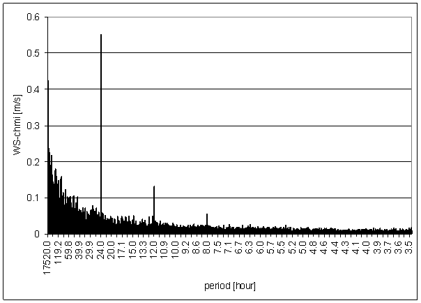
Figure 106 - WS-chmi full spectrum

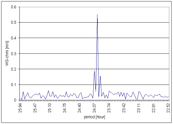
Figure 107 – 24 hour area of WS-chmi spectrum

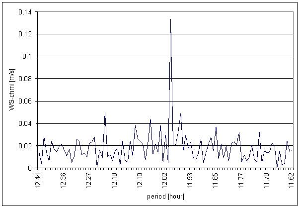
Figure 108 – 12 hour area of WS-chmi spectrum

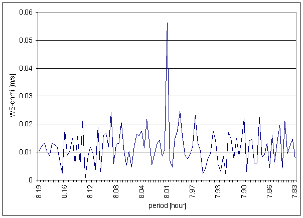
Figure 109 – 8 hour area of WS-chmi spectrum

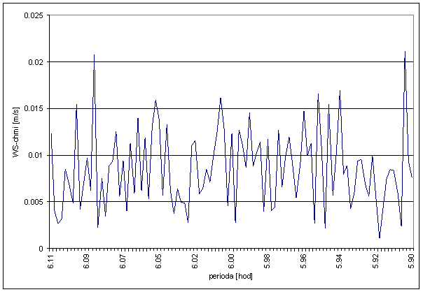
Figure 110 – 6 hour area of WS-chmi spectrum

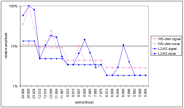
Figure 111 – Relative amplitude spectral schema of WS-chmi compared with L2-NS

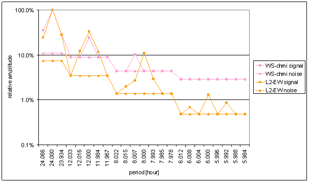
Figure 112 – Relative amplitude spectral schema of WS-chmi compared with L2-EW

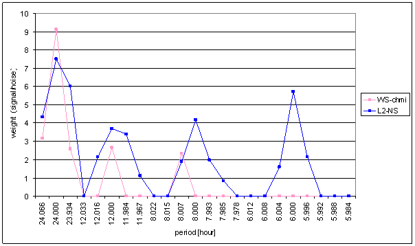
Figure 113 – Weight spectral schema of WS-chmi compared with L2-NS

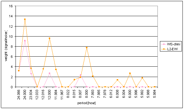
Figure 114 – Weight spectral schema of WS-chmi compared with L2-EW

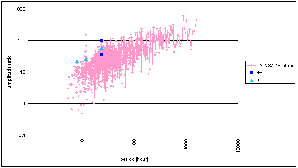
Figure 115 – Frequency characteristic of WS-chmi -> L2-NS hypothetical system

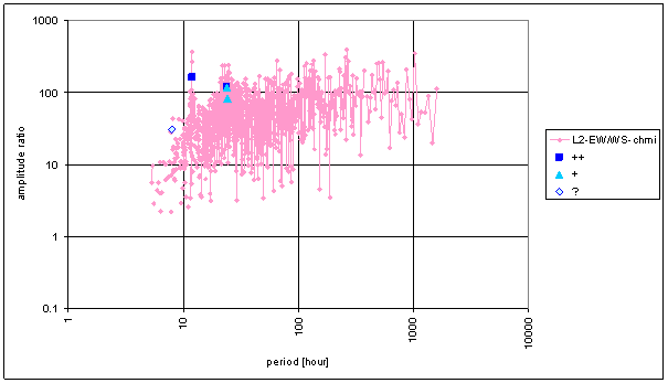
Figure 116 – Frequency characteristic of WS-chmi -> L2-EW hypothetical system

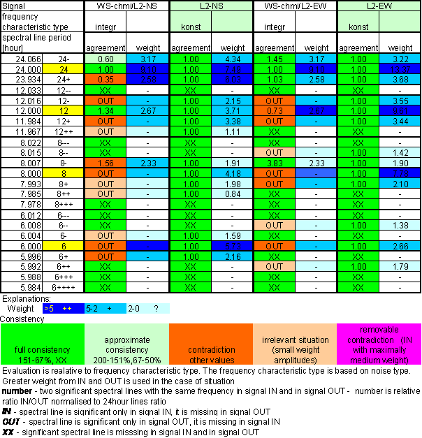
Table 19 – Correspondence evaluation of WS-chmi with L2-NS and L2-EW

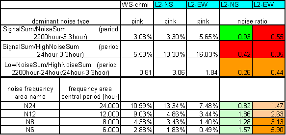
Table 20 – WS-chmi noise evaluation

The great contradiction between WS-chmi and measured displacements spectrums is result of the analysis.

Result of signal/noise evaluation is: WS-chmi can not cause L2-NS or L2-EW measured displacements.

RH-chmi

RH-chmi is air relative humidity. RH-chmi was measured by professional meteorological institute CHMI in Prague-Libuš locality by MILOS measurement system.

Measurement results have 30min time step.

The spectrum was counted from 30min averages time line in range from January 2001 to December 2002 i.e. from 35040 samples.

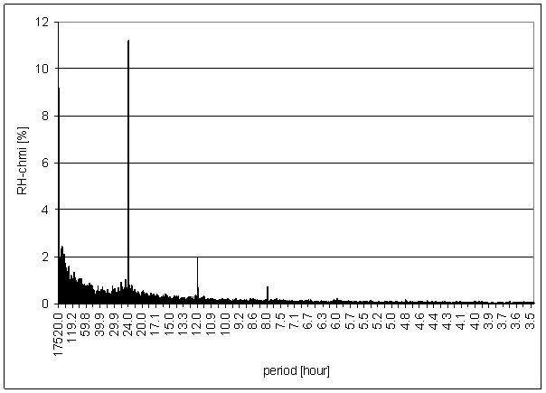
Figure 117 - RH-chmi full spectrum

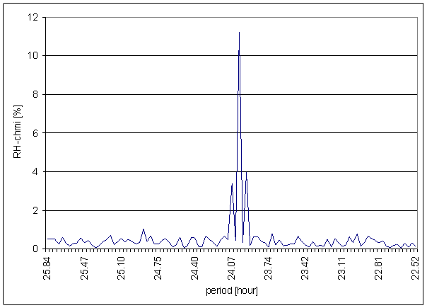
Figure 118 – 24 hour area of RH-chmi spectrum

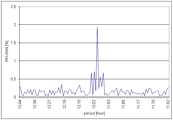
Figure 119 – 12 hour area of RH-chmi spectrum

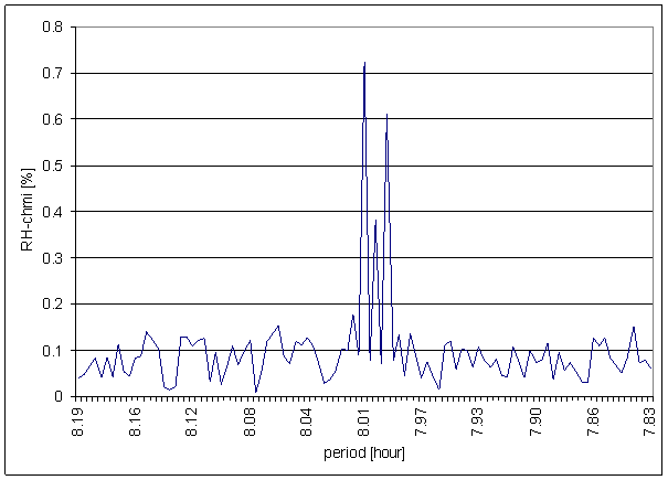
Figure 120 – 8 hour area of RH-chmi spectrum

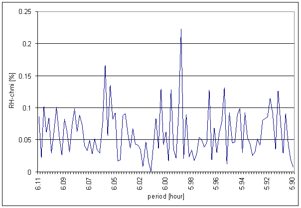
Figure 121 – 6 hour area of RH-chmi spectrum

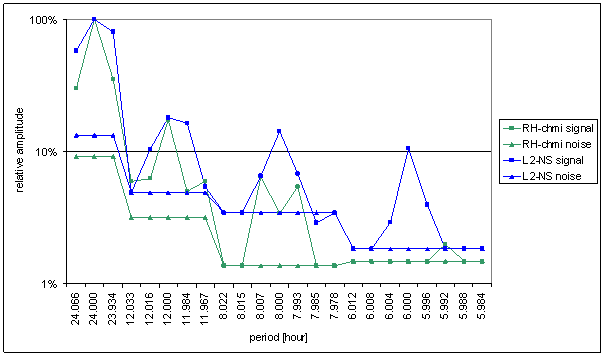
Figure 122 – Relative amplitude spectral schema of RH-chmi compared with L2-NS

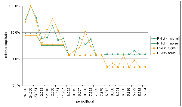
Figure 123 – Relative amplitude spectral schema of RH-chmi compared with L2-EW

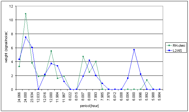
Figure 124 – Weight spectral schema of RH-chmi compared with L2-NS

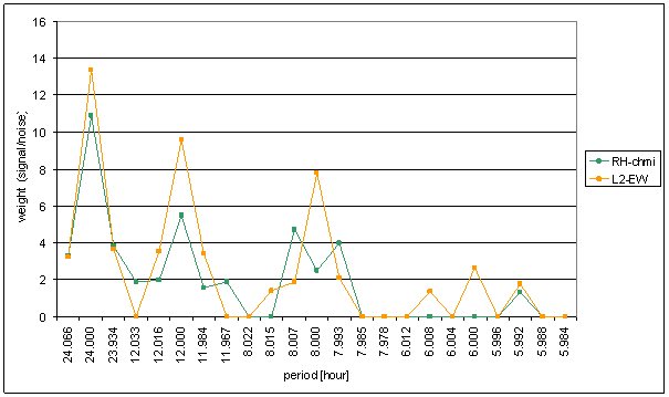
Figure 125 – Weight spectral schema of RH-chmi compared with L2-EW

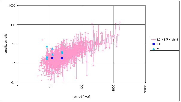
Figure 126 – Frequency characteristic of RH-chmi -> L2-NS hypothetical system

Figure 127 – Frequency characteristic of RH-chmi -> L2-EW hypothetical system

Table 21 – Correspondence evaluation of RH-chmi with L2-NS and L2-EW

Table 22 – RH-chmi noise evaluation

The great contradiction between RH-chmi and measured displacements spectrums is result of the analysis. Better correspondence results are for L2-EW spectrum than for L2-NS spectrum.

Result of signal/noise evaluation is: RH-chmi can cause L2-NS and L2-EW measured displacements.

SS

SS is theoretical Sun shine at 50° north latitude. SS was computed by numeric astronomic model of the Sun-Earth system. No atmospheric effects or no local effects were built into the model. The Earth was modelled as an ordinary sphere. No barrier was built in the model.

Model generated results have 30min time step.

The spectrum was counted from 30min averages time line in range from January 2001 to December 2002 i.e. from 35040 samples.

Figure 128 - SS full spectrum

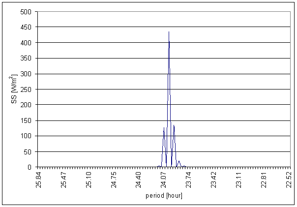
Figure 129 – 24 hour area of SS spectrum

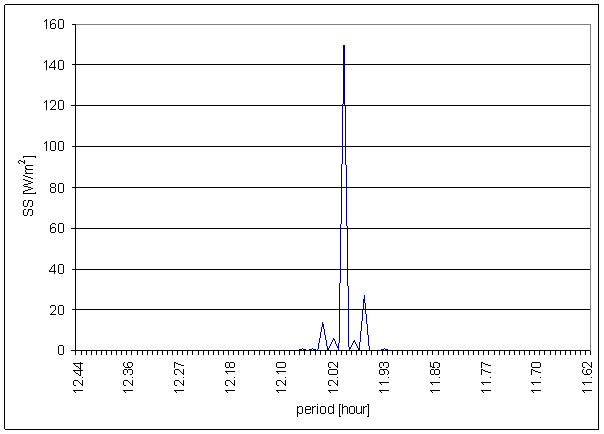
Figure 130 – 12 hour area of SS spectrum

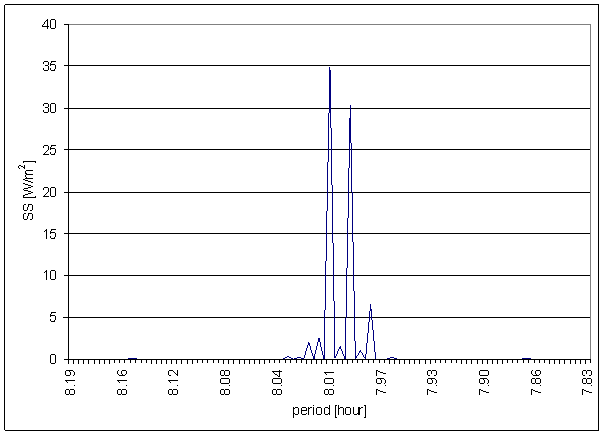
Figure 131 – 8 hour area of SS spectrum

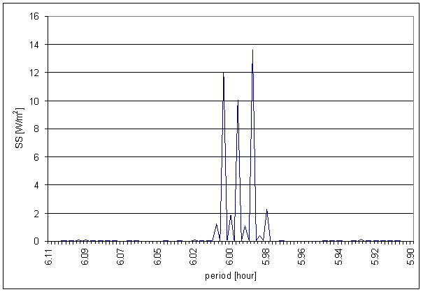
Figure 132 – 6 hour area of SS spectrum

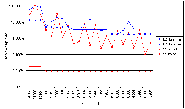
Figure 133 – Relative amplitude spectral schema of SS compared with L2-NS

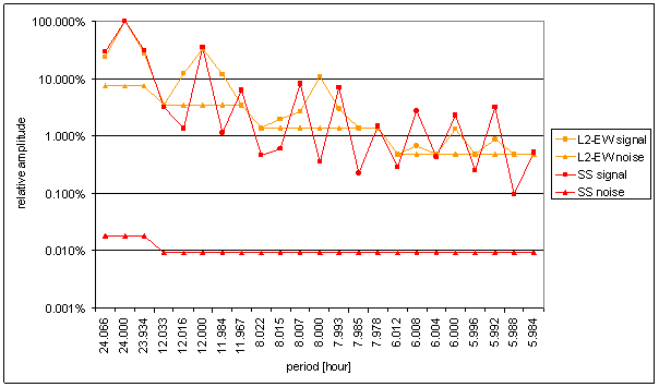
Figure 134 – Relative amplitude spectral schema of SS compared with L2-EW

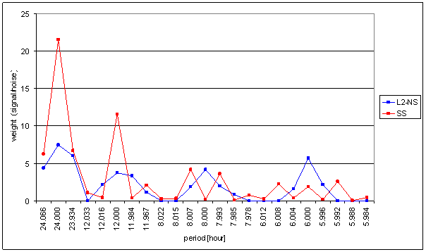
Figure 135 – Weight spectral schema of SS compared with L2-NS. Noise level from RA-chmi was used for SS weight calculation.

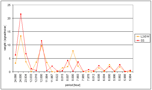
Figure 136 – Weight spectral schema of SS compared with L2-EW

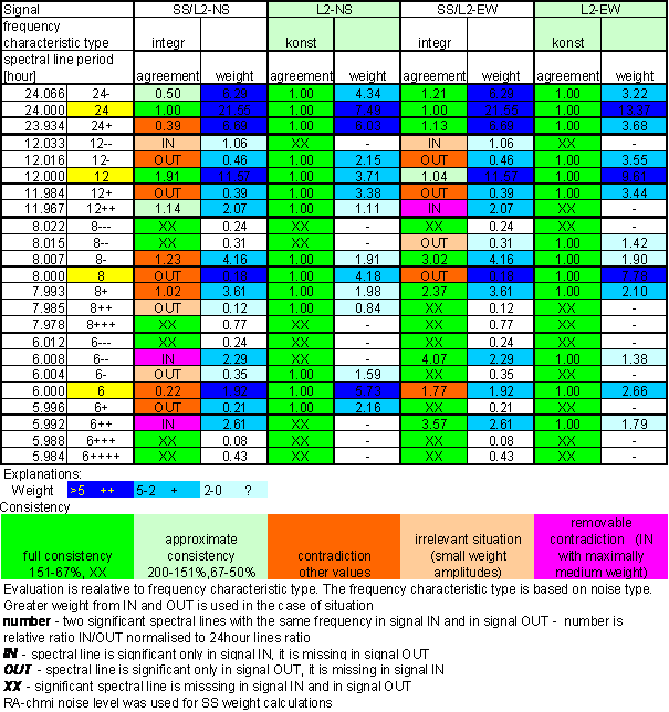
Table 23 – Correspondence evaluation of SS with L2-NS and L2-EW

The theoretical signal is presented to enable comparison with other signals, especially for comparison with measured Sun radiation RA-chmi, reconstructed Sun radiation RA-uexp and other theoretical signal SSS.

The correspondence of SS with L2-NS is very bad with respect of other signals.

The correspondence of SS with L2-EW is better than average. It is between RH-chmi and T-ext.

SSS

SSS is theoretical Sun shine with respect of local shielding at 50° north latitude. SSS was computed by numeric astronomic model of Sun-Earth system. No atmospheric effects were built into the model. The Earth was modelled as an ordinary sphere. Local shielding barrier was modelled in model to respect shielding by buildings in the L2 locality. Shielding effect was modelled by decreasing of the Sun shine to 25% of theoretical value.

The modelled buildings have two wings. One wing is in southeast direction and second one is in west direction. For more detail see Figure 244 – L2, L7 and L9 locality position schema.

Model generated results have 30min time step.

The spectrum was counted from 30min averages time line in range from January 2001 to December 2002 i.e. from 35040 samples.

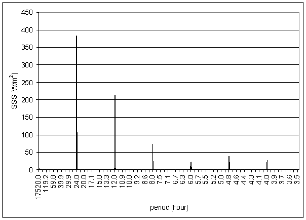
Figure 137 - SSS full spectrum

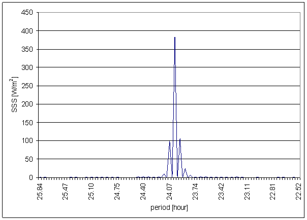
Figure 138 – 24 hour area of SSS spectrum

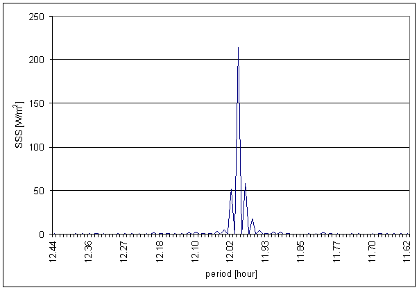
Figure 139 – 12 hour area of SSS spectrum

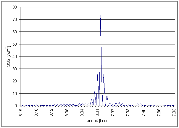
Figure 140 – 8 hour area of SSS spectrum

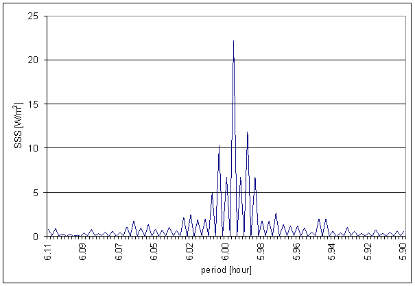
Figure 141 – 6 hour area of SSS spectrum

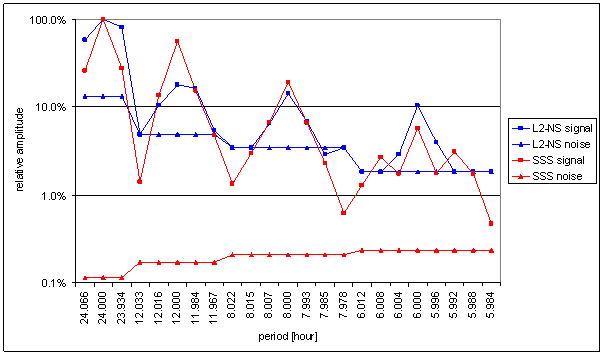
Figure 142 – Relative amplitude spectral schema of SSS compared with L2-NS

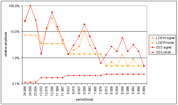
Figure 143 – Relative amplitude spectral schema of SSS compared with L2-EW

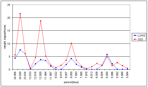
Figure 144 – Weight spectral schema of SSS compared with L2-NS. Noise level from RA-chmi was used for SSS weight calculation.

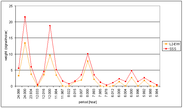
Figure 145 – Weight spectral schema of SSS compared with L2-EW

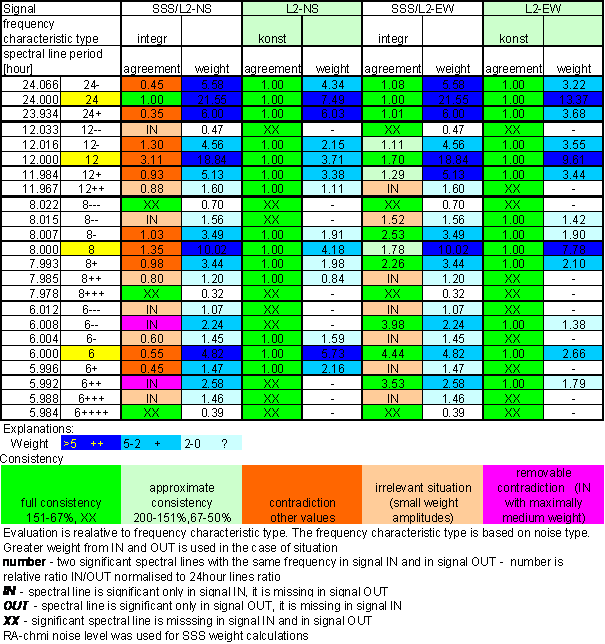
Table 24 – Correspondence evaluation of SSS with L2-NS and L2-EW

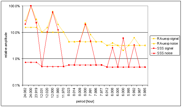
Figure 146 – Relative amplitude spectral schema of SSS compared with RA-uexp

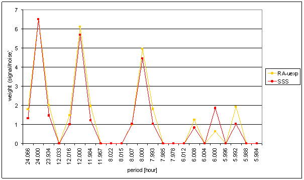
Figure 147 – Weight spectral schema of SSS compared with RA-uexp. Noise level from RA-uexp was used for SSS weight calculation.

SSS and RA-uexp spectrum comparison shows difference between these signals.

The theoretical signal SSS is presented to enable comparison with other signals. Especially for comparison with measured Sun radiation RA-chmi, reconstructed Sun radiation RA-uexp and other theoretical signal SS.

The correspondence of SSS with L2-NS is very bad with respect of other signals. It gives the worst results from all compared signals (counted as sum of identical and sum of contradictory spectral line ratio)

The correspondence of SSS with L2-EW has the best level from all external effects (together with RA-uexp and intRA-uexp). Integrating frequency characteristics for correspondence evaluation had to be used.

Modelled SSS signal does not contain cloudiness and temperature effects. It contains only local shielding effects and the Sun-Earth geometry.

Measured and reconstructed RA-uexp signal contains temperature, cloudiness, the Sun-Earth geometry and local shielding impacts.

Modelled SS signal does not contain cloudiness, temperature and local shielding impacts. It contains only the Sun-Earth geometry.

Measured RA-chmi signal contains cloudiness effect and the Sun-Earth geometry effect. It does not contain local shielding and temperature effects.

SSS and RA-uexp frequency spectrums are the closest to L2-EW spectrum.

SS and RA-chmi spectrum correspondence with L2-EW spectrum is not very good.

Conclusions are:

Geometrical local shielding effect is important effect of SSS, RA-uexp and L2-EW signals.
Cloudiness has no significant effect to SSS, RA-uexp and L2-EW spectrums.

L2-NS

L2-NS is north-south component of measured displacements in L2 locality.

Measurement was made every 15sec in two orthogonal coordinates in one step. Primary measurement results were transformed to north-south and east-west directions by rotation and scale factor multiplication.

The spectrum was counted from 30min averages time line in range from January 2001 to December 2002 i.e. from 35040 samples. The spectrum was used for comparison with other signal spectrums in the same range.

Figure 148 – L2-NS full spectrum

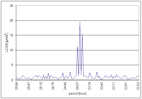
Figure 149 – 24 hour area of L2-NS spectrum

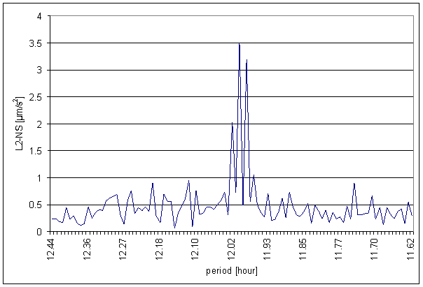
Figure 150 – 12 hour area of L2-NS spectrum

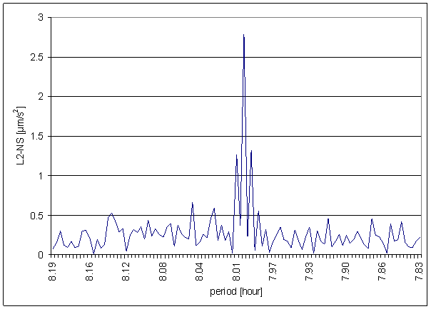
Figure 151 – 8 hour area of L2-NS spectrum

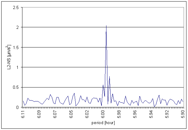
Figure 152 – 6 hour area of L2-NS spectrum

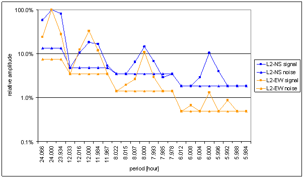
Figure 153 – Relative amplitude spectral schema of L2-NS compared with L2-EW

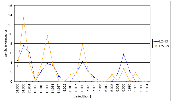
Figure 154 – Weight spectral schema of L2-NS compared with L2-EW

Figure 155 – Frequency characteristic of L2-NS -> L2-EW hypothetical system. Frequency characteristic of hypothetical system between two orthogonal components of one measured displacement vector.

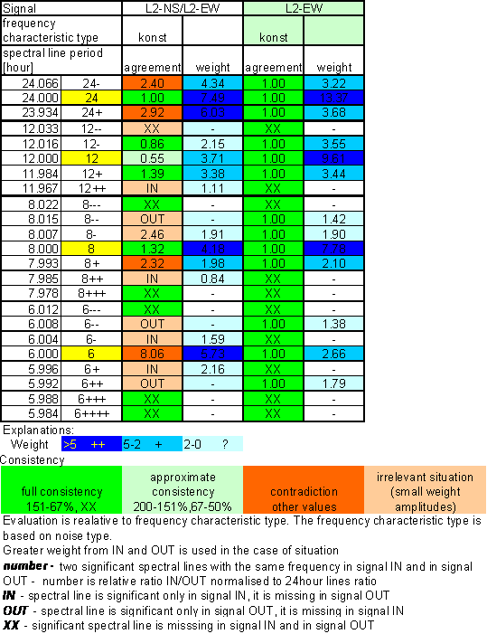
Table 25 – Correspondence evaluation of L2-NS with L2-EW

Table 26 – L2-NS and L2-EW noise evaluation

The following spectrum was counted from 30min averages time line in range from September 2001 to March 2003 i.e. from 28320 samples. The spectrum was used for comparison with other signal spectrums in the same range.

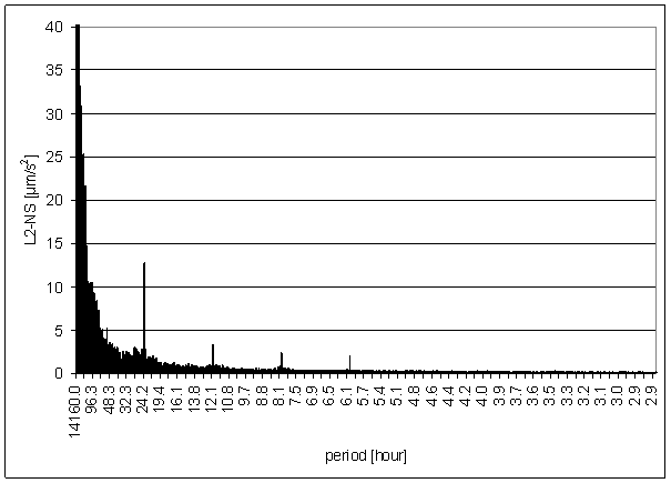
Figure 156 – L2-NS full spectrum

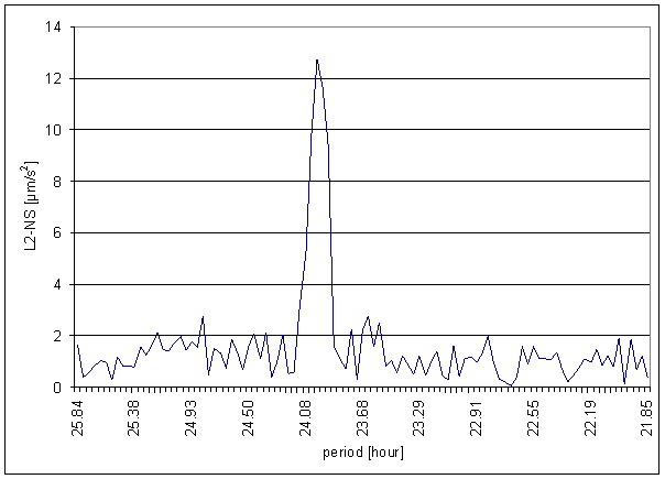
Figure 157 – 24 hour area of L2-NS spectrum

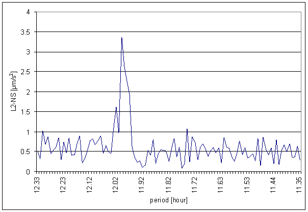
Figure 158 – 12 hour area of L2-NS spectrum

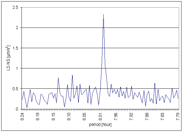
Figure 159 – 8 hour area of L2-NS spectrum

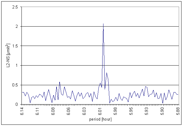
Figure 160 – 6 hour area of L2-NS spectrum

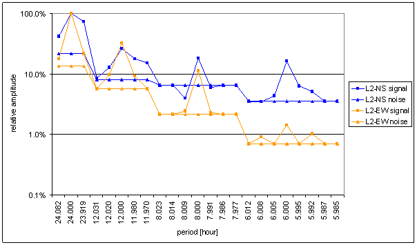
Figure 161 – Relative amplitude spectral schema of L2-NS compared with L2-EW

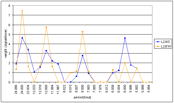
Figure 162 – Weight spectral schema of L2-NS compared with L2-EW

L2-NS and L2-EW comparison shows great difference in spectrum of these orthogonal components of measured displacements. It is not possible to implement any linear system with constant parameters to convert L2-NS into L2-EW spectrum (e.g. see spectral line 6).

These two components partially differ in noise spectrum. It can be seen form hypothetical system frequency characteristics.

L2-EW

L2-EW is east-west component of measured displacements in L2 locality.

Figure 163 – L2-EW full spectrum

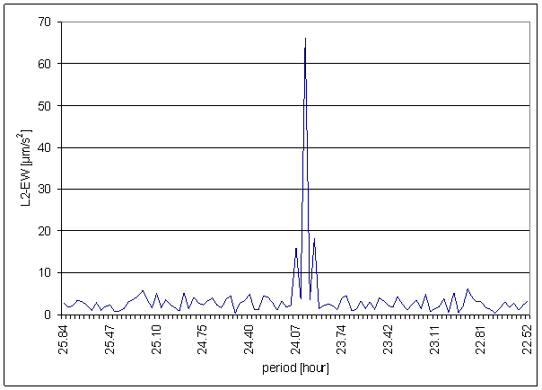
Figure 164 – 24 hour area of L2-EW spectrum

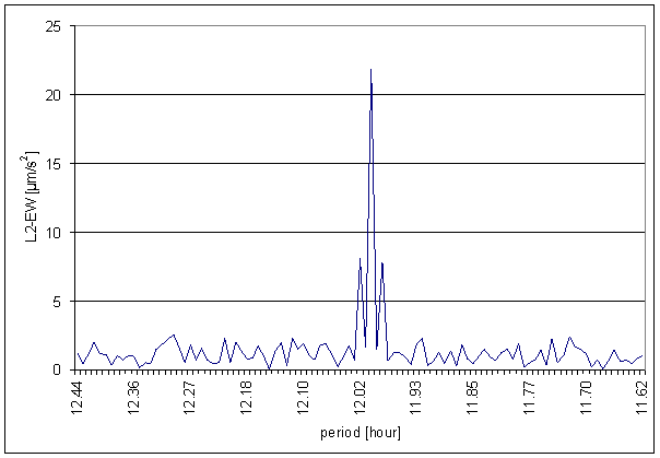
Figure 165 – 12 hour area of L2-EW spectrum

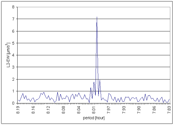
Figure 166 – 8 hour area of L2-EW spectrum

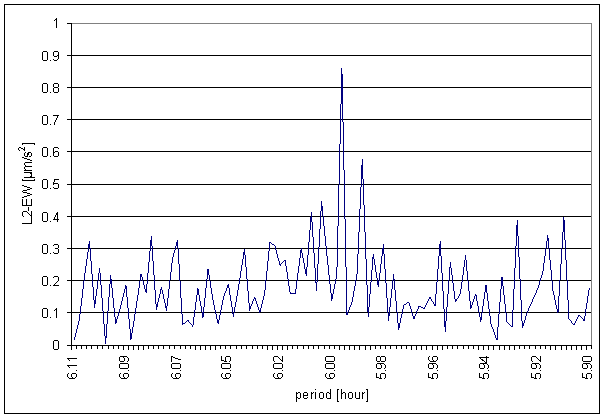
Figure 167 – 6 hour area of L2-EW spectrum

Figure 168 – Relative amplitude spectral schema of L2-EW compared with L2-NS

Figure 169 – Weight spectral schema of L2-EW compared with L2-NS. The schema is equivalent to the one from previous section due to symmetry.

Figure 170 – Frequency characteristic of L2-EW -> L2-NS hypothetical system. Frequency characteristic of hypothetical system between two orthogonal components of one measured displacement vector. It is inverse characteristic to the one in previous section.

Table 27 – Correspondence evaluation of L2-EW with L2-NS

Figure 171 – L2-EW full spectrum

Figure 172 – 24 hour area of L2-EW spectrum

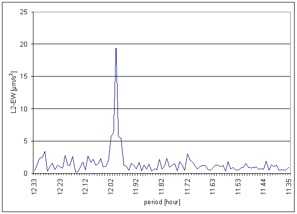
Figure 173 – 12 hour area of L2-EW spectrum

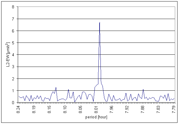
Figure 174 – 8 hour area of L2-EW spectrum

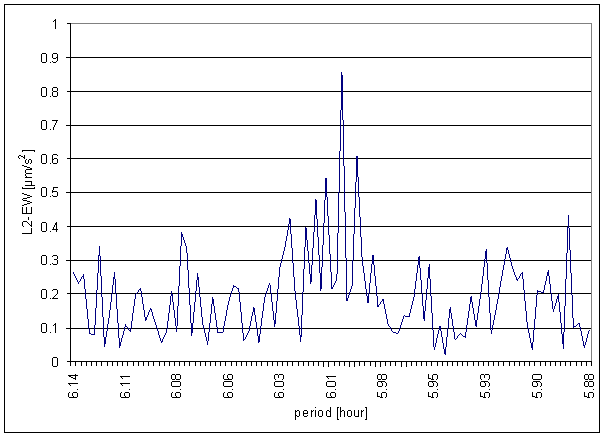
Figure 175 – 6 hour area of L2-EW spectrum

Figure 176 – Relative amplitude spectral schema of L2-EW compared with L2-NS

Figure 177 – Weight spectral schema compared of L2-EW with L2-NS

L2-NS and L2-EW comparison imply the fact, that these orthogonal components of measured displacements can not have one simple local common cause.

The cause can not be any scalar. The cause can not be any vector with the same frequency spectrum of its components.

The cause can be only vector with different frequency spectrum of the components or combination of two or more causes. Composition of causes must be done this way, that one component must be exactly in north-south direction.

Note: L2-NS contains spectral line 6 and L2-EW does not contain this line. If the direction of cause with spectral line 6 is different from north-south direction, spectral line 6 must be visible in east-west component spectrum.

Combination of impacts

The hypothesis based on idea, that measured displacements are caused by response of linear dynamic system with constant parameters stimulated by linear combination of two or more external effect signals, is studied in this section.

Special features of spectral lines combinations are important in this hypothesis.

Any combinations of any signals can not cause new frequency in linear systems.

Some spectral line can disappear only on very specific circumstances:

Can be overlapped by noise
Can disappear by sum of two exactly synchronous signals with opposite phases
Site spectral lines can disappear by sum of two synchronous signals with synchronous opposite modulation phases

Let us try to find combination of external effect signals to generate spectrum similar to measured displacements spectrum.

The success is essential condition but not sufficient condition. The non-success is sufficient condition to prove the hypothesis invalidity.

The validity criterion is at least approximate consistency of exactly all spectral lines of periodic signal spectral parts. Noise spectral parts are not included in the validity criterion.

The approximate consistency is defined as in previous sections i.e. as the case if two compared signals have spectral lines with exactly the same frequency and amplitudes are approximately each other, it means the amplitudes do not differ more than 50% with respect to the greater ones (-50% to +100% with respect to selected signal).

The hypothetical linear system can have different frequency characteristics for every input signal. The frequency characteristics must be the same for periodic signal spectral lines and for surrounding noise. It means the spectral line weight is independent on frequency characteristics of the hypothetical system.

The hypothesis testing is based on weight spectral line analysis in the first step.

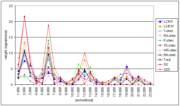
Figure 178 – Weight spectral schema of external effects and measured displacements– range January 2001 – December 2002

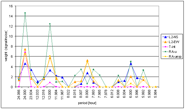
Figure 179 – Weight spectral schema of external effects and measured displacements– range September 2001 – March 2003

Basic difference of all external signal weight spectral lines and measured displacements L2-NS and L2-EW ones in 8hour a 6hour areas can be recognized. Good consistency in these areas is essential condition for hypothesis success. Bad consistency in these areas causes hypotheses failure.

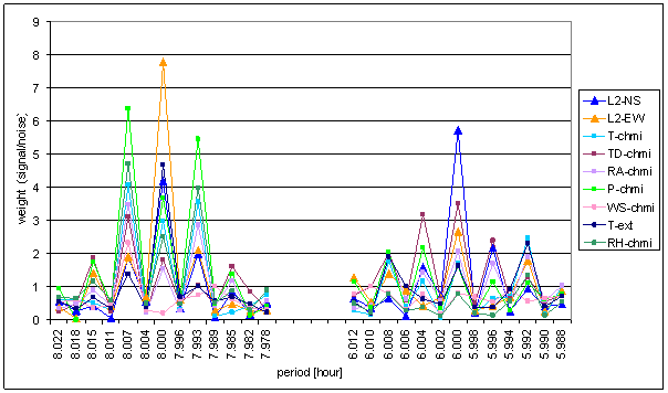
Figure 180 – Weight spectral schema selected part of external effects and measured displacements– range January 2001 – December 2002

The selected weight spectrum shows the fact, that there is no external effect signal containing spectral line 6 with weight comparable with L2-EW. The 8hour area is more complicated.

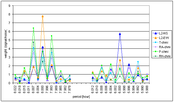
Figure 181 – Weight spectral schema selected part of external effects T-chmi, RA-chmi, P-chmi, RH-chmi and measured displacements– range January 2001 – December 2002

There is no external effect signal with weight greater or equal to L2-EW 8hour spectral line weight. Signals T-chmi, RA-chmi, P-chmi and RH-chmi contain spectral lines 8- and 8+ with great weight. These spectral lines can be site spectral line of basic line 8. Combinations of these signals can theoretically compensate modulation. Compensated modulation signal has greater central spectral line and small or none site spectral lines.

Figure 182 – Weight spectral schema selected part of external effects T-ext, TD-chmi, WS-chmi and measured displacements– range January 2001 – December 2002

Signals T-ext, TD-chmi and WS-chmi have only small weight of site spectral lines and small weight of central line. No combination of these signal can give cause L2-EW 8hour spectral line.

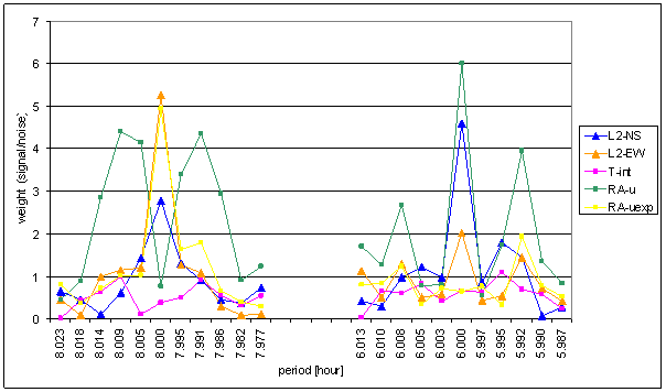
Figure 183 – Weight spectral schema selected part of external effects and measured displacements– range September 2001 – March 2003

Signal RA-uexp spectrum is very similar to L2-EW measured displacements one in 8hour spectral area. There is no other signal to be combined with. All other signals have lower weight. Any combination of RA-uexp with these signals must give sum with lower weight than RA-uexp itself.

Signal RA-u is the only signal containing spectral line 6hour with greater weight than L2-NS spectrum. RA-u contains spectral lines 6-- and 6++ with great weight. These lines can be site lines of highly modulated 6hour periodic signal.

RA-u is artificial signal. It is generated by nonlinear transformation of physical external effect (Sun radiation logarithm). This signal can not cause measured displacements. The measured displacements L2-NS and L2-EW had been measured several months before the RA-u generating measured device was designed and built.

The previous analyses give following partial results:

There is no external effect signal containing spectral line 6.00hour with great signal/noise ratio to can cause L2-NS component of measured displacements.
There is a chance, that only T-chmi, RA-chmi, P-chmi and RH-chmi can be combined some way to give result comparable with 8hour spectrum of L2-EW component of measured displacement. The combination must “compensate” 8++ and 8-- spectral lines and increase signal/noise ratio of 8 spectral line.

This is one of the reasons why time dependency of spectrum is analyzed in the next section.

Spectrum time dependency

Some separated results of spectrum time dependency analysis are presented in this section. Analyses were made by STFT [6, 7]. Cosines sliding window using 4608 samples (30min) i.e. 96 days was used. Time axis displayed date is date of the window centre.

Previous section analysis results shows the best similarity between total spectrums of measured displacements in L2 locality and total spectrums of measured sunshine (RA-uexp, RA-chmi), simulated sunshine (SS, SSS) and external temperature (T-ext, T-chmi). Following figures display spectrum time dependency of these signals.

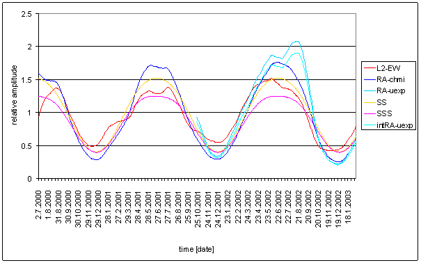
Figure 184 – 24hour spectral line time dependency of Sun radiation (RA-chmi, RA-uexp, SS, SSS, and intRA-uexp) and L2-EW

Every spectral line is relative to its 24hour spectral line average value. Let us note different noise type of measured displacement (pink) and Sun radiation (white). The fact must be taken into account in the result analysis. Spectral lines of high frequency have amplitude proportionaly lower in case of integrating frequency characteristics.

Signal intRA-uexp is numericaly integrated signal RA-uexp.

Figure 185 – 12hour spectral line time dependency of Sun radiation (RA-chmi, RA-uexp, SS, SSS, and intRA-uexp) and L2-EW

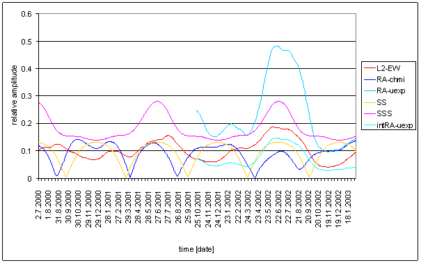
Figure 186 – 8hour spectral line time dependency of Sun radiation (RA-chmi, RA-uexp, SS, SSS, and intRA-uexp) and L2-EW

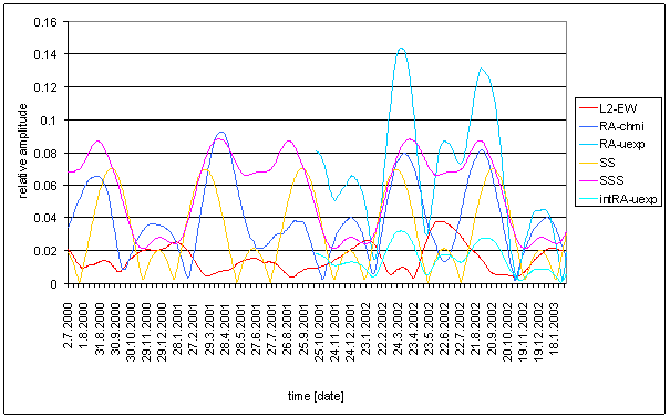
Figure 187 – 6hour spectral line time dependency of Sun radiation (RA-chmi, RA-uexp, SS, SSS, and intRA-uexp) and L2-EW

Figure 188 – 24hour spectral line time dependency of external temperature (T-chmi, T-ext) and L2-EW

Figure 189 – 12hour spectral line time dependency of external temperature (T-chmi, T-ext) and L2-EW

Figure 190 – 8hour spectral line time dependency of external temperature (T-chmi, T-ext) and L2-EW

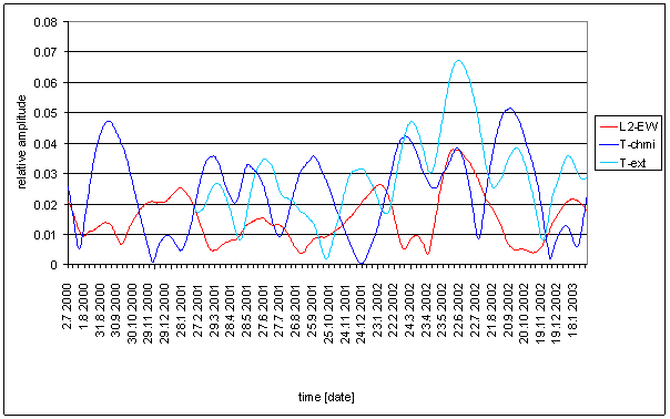
Figure 191 – 6hour spectral line time dependency of external temperature (T-chmi, T-ext) and L2-EW

The spectral line time dependency analysis results supports conclusions of total spectrum analysis from other point of view and give additional facts.

Basic consistency of 24.00 hour spectral lines time dependency of all analyzed signal was verified. Detail analysis shows differences. Rising and falling edges in year 2002 of L2-EW precede other signals about 15 - 25 days in equinox time area.

Time dependency of 12.00 hour spectral lines shows great differences. T-ext and T-chmi have clear 2 periods per year. RA-chmi and SS have half year period too. Only RA-uexp and SSS have similar time dependency to L2-EW.

Time dependency of 8.00 hour spectral lines gives other results. RA-chmi, SS and T-chmi signals have spectral characteristic time dependency with periodic falling close to zero amplitude close to equinox time. It is characteristics of 3rd harmonics disappearing in exactly half wave sinusoidal signal. This effect is typical to direct Sun exposure of ideal earth surface.

RA-uexp, SSS, T-ext and L2-EW signals have quite different time dependency. They have only one maximum per year and they have no situation with values close to zero.

T-ext has opposite phase of spectrum time dependency with respect of L2-EW one. If T-ext has maximum, L2-EW has minimum and vice versa.

Only L2-EW, RA-uexp and SSS have similar time dependency of 8.00 hour spectral lines.

No conclusions can be made form 6.00 hour spectral lines. The signals have great noise nature.

The analysis results give conclusions:

RA-chmi, SS, T-chmi and T-ext can not be local cause of L2-EW measured displacements. This is valid in case of linear dynamic system with constant parameters hypothesis and in case of nonlinear static system with constant parameters hypothesis.
Only SSS and RA-uexp signals have similar time dependency to L2-EW for all spectral lines that causality can be supposed (if prematureness is omitted). They have 12.00hour and 8.00 hour spectral lines different amplitudes and different noise type than L2-EW. The best correspondence to L2-EW gives intRA-uexp signal.

Similar analysis for L2-NS measured displacements (perpendicular) component is in following text.

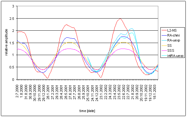
Figure 192 – 24hour spectral line time dependency of Sun radiation (RA-chmi, RA-uexp, SS, SSS, and intRA-uexp) and L2-NS

Figure 193 – 12hour spectral line time dependency of Sun radiation (RA-chmi, RA-uexp, SS, SSS, and intRA-uexp) and L2-NS

Figure 194 – 8hour spectral line time dependency of Sun radiation (RA-chmi, RA-uexp, SS, SSS, and intRA-uexp) and L2-NS

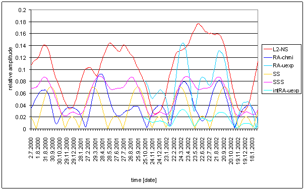
Figure 195 – 6hour spectral line time dependency of Sun radiation (RA-chmi, RA-uexp, SS, SSS, and intRA-uexp) and L2-NS

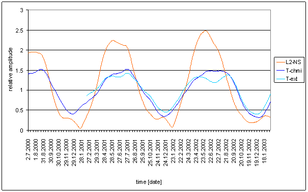
Figure 196 – 24hour spectral line time dependency of external temperature (T-chmi, T-ext) and L2-NS

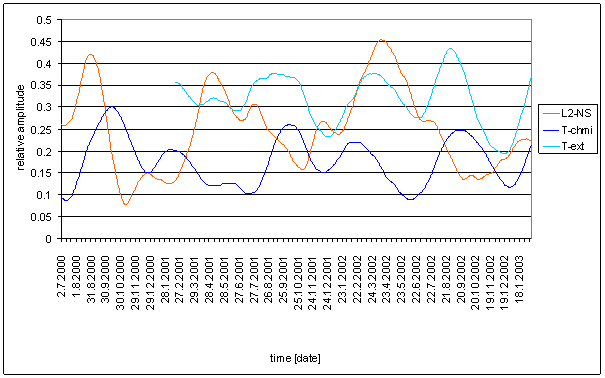
Figure 197 – 12hour spectral line time dependency of external temperature (T-chmi, T-ext) and L2-NS

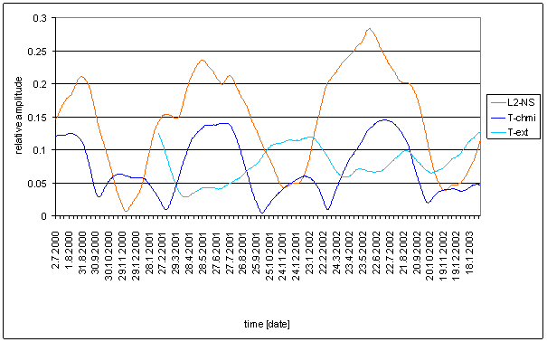
Figure 198 – 8hour spectral line time dependency of external temperature (T-chmi, T-ext) and L2-NS

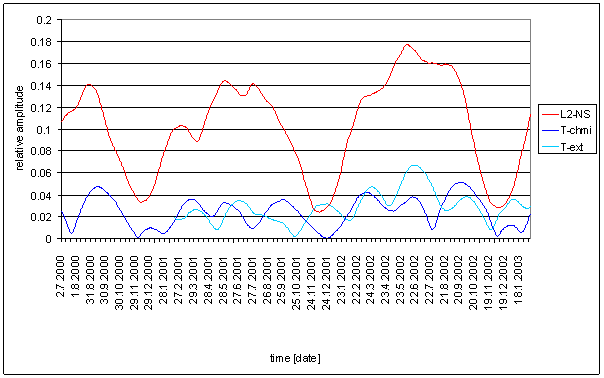
Figure 199 – 6hour spectral line time dependency of external temperature (T-chmi, T-ext) and L2-NS

Time dependency of 24.00 hour spectral lines shows difference between L2-NS and other analyzed external effects time dependency. The difference is greater than difference in case L2-EW.

Time dependency of 12.00 hour spectral lines of L2-NS shows one maximum per year. T-ext, T-chmi, RA-chmi and SS have clear 2 periods per year. RA-chmi can be supposed to be similar to L2-NS in the year 2001. It is not true in the year 2002.

RA-uexp, intRA-uexp and SSS time dependence shows important time shift against L2-NS one.

Time dependency of 8.00 hour spectral line of L2-NS is quite different than other signals time dependency spectral lines. It has significantly greater amplitude than RA-chmi, intRA-uexp, SS, T-chmi and T-ext signals. Only SSS has comparable maximum amplitude. But SSS minimum amplitude is not comparable with L2-NS minimum amplitude. RA-uexp has greater maximum amplitude than L2-NS, but other noise type.

Time dependency of L2-NS 6.00 hour spectral line is essentially different than all compared ones. No other signal has the same amplitude or the similar amplitude time dependency slope.

The analysis results give these conclusions. Any analyzed signal can not be local cause of L2-NS measured displacements. This is valid in case of linear dynamic system with constant parameters hypothesis and in case of nonlinear static system with constant parameters hypothesis.

Let us return to the linear combinations of T-chmi, RA-chmi, P-chmi and RH-chmi in 8.00 hour spectral area hypothesis. Can be some linear combinations of these signals similar to L2-EW spectrum time dependency?

Spectral line time dependencies of all these signals are on the following figure.

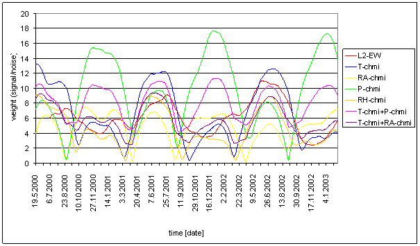
Figure 200 – 8hour spectral line time dependency of external effects (T-chmi, RA-chmi, P-chmi, and RA-chmi), combination of external effects T-chmi+P-chmi, T-chmi+RA-chmi and measured displacements L2-NS. All signals are standardized to the maximum noise level of the particular signal in 8hour area with respect of global spectrum.

L2-EW and hypothetical T-chmi+P-chmi and T-chmi+RA-chmi sums are displayed in the figure. The displayed sums are the best ones from all other combinations with respect of spectral lines time dependency “phase” or time shifts.

Every compared external effects signal have sharp minimum close to equinox. Every sum has the equinox minimums too. But L2-EW has no equinox minimum. L2-EW amplitude minimum is close to winter solstice. Every compared external effects signal sum has local maximum close to winter solstice.

Every sum has two maximums per year but L2-EW has only one maximum per year.

Similar results give sums of three or all signals.

Analysis result is: Any linear combination of T-chmi, RA-chmi, P-chmi and RH-chmi signals can not give signal with similar spectrum time dependency to L2-EW one in 8 hours spectral area. Previous section excluded other signals due to signal/noise ratio.

Other external effects signals spectrum time dependency is shown in following figures for completeness.

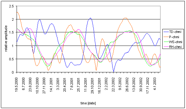
Figure 201 – 24hour spectral line time dependency of external effect TD-chmi, P-chmi, WS-chmi and RH-chmi

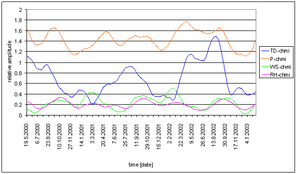
Figure 202 – 12hour spectral line time dependency of external effect TD-chmi, P-chmi, WS-chmi and RH-chmi

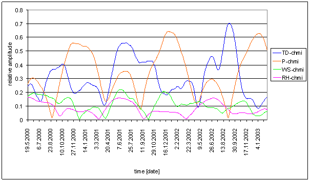
Figure 203 – 8hour spectral line time dependency of external effect TD-chmi, P-chmi, WS-chmi and RH-chmi

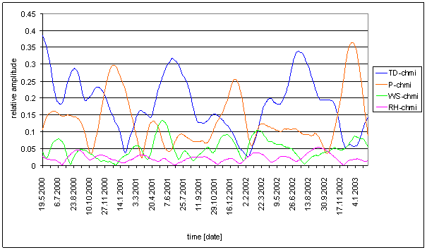
Figure 204 – 6hour spectral line time dependency of external effect TD-chmi, P-chmi, WS-chmi and RH-chmi

Time dependency of TD-chmi, P-chmi, WS-chmi and RH-chmi spectrums are essentially different from L2-NS and L2-EW ones at least in one spectral area.

Any of TD-chmi, P-chmi, WS-chmi and RH-chmi signal can not be local cause of L2-NS measured displacements.

Summary

Following summary tables recapitulate spectrum comparisons from previous sections.

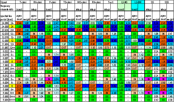
Table 28 – Aggregated correspondence evaluation of L2-NS from range January 2001 – December 2002

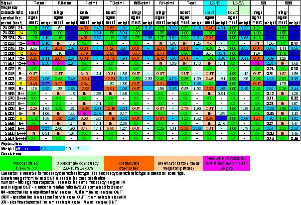
Table 29 – Aggregated correspondence evaluation of L2-EW from range January 2001 – December 2002

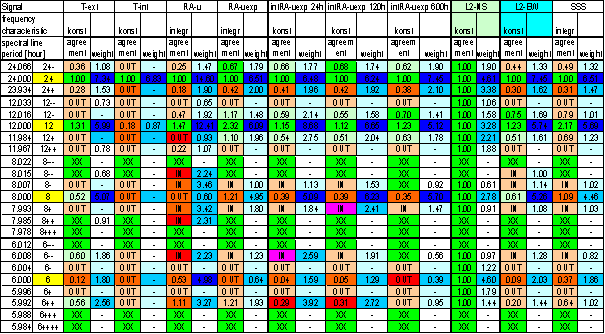
Table 30 – Aggregated correspondence evaluation of L2-NS from range September 2001 – March 2003

Table 31 – Aggregated correspondence evaluation of L2-EW from range September 2001 – March 2003

Global spectrums comparison results are in following summary:

Compared signals global nature is similar. All signals contain periodical signal with 24.00 hour basic period and its higher harmonics with site spectral lines. All signals contain high irregular part that can be supposed to be a noise.
Any signal does not contain any other strong periodical component

Most of signals contain pink noise (1/f) or similar. Only Sun radiation signals contain white noise (frequency almost independent)
Signals P-chmi, TD-chmi, WS-chmi and T-int have very low signal/noise ratio so they can not cause the measured displacements signals. The signal/noise ratios are minimally 30% lower than relevant L2-NS and L2-EW ones.
T-chmi, RA-chmi, RH-chmi, T-ext, RA-u and RA-uexp signals have signal/noise ratio comparable with measured displacements L2-NS and L2-EW ones. L2-EW signal has maximal signal/noise ratio in 24hour-3.3hour area from all signals.
No analyzed external effect signal has spectral features to enable safely prove equivalence with at least one measured displacements component. Some spectral line exists in all cases, which are out of wide tolerance area -50% +100%.

The best correspondence between measured displacements component and external effect signal is between RA-uexp and L2-EW and between SSS and L2-EW. Integrating frequency characteristics of hypothetical linear system must be taken into account. The integration must be minimally in spectral range 300hour to 3hour. This conclusion was proved by good correspondence of numerically integrated signal intRA-uexp.
The comparison time range of RA-uexp was only 1.6 year. Other signals used 2year time range. The comparison of RA-uexp can be influenced by greater error than in case of longer comparison time range.
T-ext and RA-chmi external effect signals gives the best correspondence with L2-EW from all directly measured external effects signals. RA-uexp was not directly measured.
No measured external effects signals have good correspondence with L2-NS. All correspondences are worse than correspondence L2-EW with L2-NS.
T-chmi, P-chmi, TD-chmi and RH-chmi external effects signals have too bad correspondence with L2-NS and L2-EW and can not be cause of measured displacements.
Different measured displacements components L2-NS and L2-EW have very different period signal spectrums and partially different noise spectrums. The greatest difference is in case of 6.00 hour spectral lines. The 6.00hour spectral line is important spectral line of L2-NS spectrum but negligible spectral line in L2-EW spectrum (signal/noise ratio is close to 1).

From the first approximation point of view external temperature (T-ext and T-chmi) and Sun radiation (RA-chmi, RA-uexp) can be supposed to be the most probable input of hypothetical local dynamic linear system driving measured displacements in L2 locality.

All other external effects signals must be excluded. The reason is bad spectrum correspondence or low signal/noise ratio or both.

Spectral analysis shows, that both orthogonal synchronously measured displacements components cannot have common scalar cause. They have very different global spectrums and very different spectrum time dependence. External temperature cannot be the only cause of measured displacements. Only Sun radiation or external temperature with Sun radiation can be probable cause of measured displacements.

L2-NS spectrum contains very strong 6.00hour spectral line. No other spectrum contains this strong spectral line (not even L2-EW spectrum). Only RA-u spectrum contains great spectral lines in 6hour spectral area. This signal contains other spectral lines 6-- and 6++. This site spectral lines mean different spectrum time dependency. RA-u spectrum time dependency analysis show two maximums and two minimums per year. The maximums are close to equinox and the minimums are close to solstice. This is quite different from L2-NS 6hour spectral line time dependency.

RA-u signal is artificial nonlinear signal with no physical meaning. The signal did not exist during whole L2 displacement measuring time. This signal can not cause measured displacements. RA-uexp does not contain this strong spectral line.

Modelled theoretical signals SS and SSS contain 6hour spectral line too. Relative amplitude (with respect of integrating dynamic system frequency characteristics) is not comparable with L2-NS 6hour spectral line and spectrum time dependences are different too.

Hypothetical possibility of T-chmi, RA-chmi, P-chmi, and RH-chmi signals linear combinations is impossible. Combination with other external effects signal is impossible due to low signal/noise ratio. Any combination has other 8hour spectrum time dependency than L2-EW.

Spectrum time dependency comparisons verified previous conclusions.

The best spectrum time dependency correspondences are between RA-uexp (and modelled SSS) and L2-EW. These two signals include local Sun movement geometry in L2 locality. The integrating frequency characteristics must be used for comparison. It proves intRA-uexp signal.

L2-NS spectrum time dependency is not comparable with any other external effect signals.

L2-EW 24.00 hour spectral lines time dependency analysis shows time difference of rising and falling edges. It shows 15 to 25 days prematureness of L2-EW before RA-uexp signals in year 2002 equinox time. This prematureness does not allow direct local dependency of L2-EW on RA-uexp respectively on Sun radiation in L2 locality.

Any external effect or any linear combination of external effects can not be cause of measured displacements if linear dynamic system with constant parameters is considered.

The best correspondence of L2-EW measured displacements component with the Sun relative movement (with respect of the signal time integral) in measurement locality (RA-uexp, SSS) and bad correspondence of the same physical quantity from close but another locality (RA-chmi, SS) gives hypothesis, that measured displacements are influenced by building geometry in L2 locality surrounding.

Nonlinear static system with constant parameters

Nonlinear hypothetical system analyzed in this section is supposed to be a static system with constant parameters. It means that the system has no significant dependency of output on input history and the system behaviour is time independent. The system gives the same result for the same stimulation any time.

Eventual small influence dynamic impacts (less than approx. 30% of total signal) are supposed to be negligible. The analysis goal is not to find parameter values for good approximation, but answer the question, if the system exists or not.

Dynamic impacts outside analyzed spectral area are negligible too. It means dynamic impacts with period shorter than 3.5 hour (mulitiminute and shorter processes) and longer than 2200 hour (mulitimonth, year and longer processes).

The working hypothesis can be formulated with previously described limits in the mind. Measured displacements are caused by some external effects itself or by combination of more external effects. General time independent nonlinear function f exists describing the hypothetical system transfer function, where y is output signal and x is input signal.

All analyzed signals have very irregular waveform. The waveform contains periodic component with basic period 24hour and its higher harmonics. The harmonic signal amplitude is not constant. Harmonic signal amplitude is time dependent. The analysis must count with irregular component and with periodic component with variable amplitude.

Irregular component was supposed to be a noise in frequency spectral analysis in previous sections. In this section dealing with nonlinear effects must be analyzed other way.

Irregular component was computed as sliding 15 days average. All signals were computed the same way. This irregular component computing method eliminates all periodic elements with periods shorter or equal to 24 hour in all signals with periodic element smaller than irregular element. Average value close to periodic signal average value is result of other signals (e.g. RA-chmi) computation.

Irregular component time dependencies of compared signals are displayed in following figures.

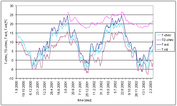
Figure 205 – Time dependence of T-chmi, TD-chmi and T-int irregular component

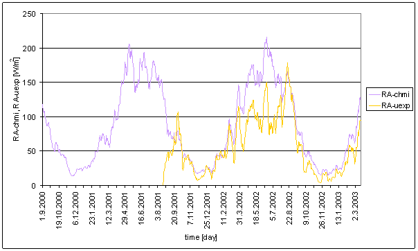
Figure 206 – Time dependence of RA-chmi and RA-uexp irregular component

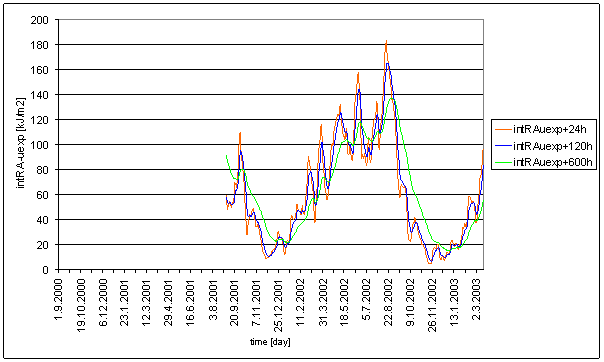
Figure 207 – Time dependence of intRA-uexp t=24hour, intRA-uexp t=120hour and intRA-uexp t=600hour irregular component

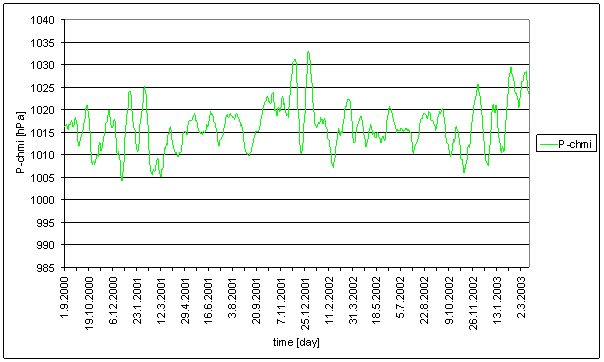
Figure 208 – Time dependence of P-chmi irregular component

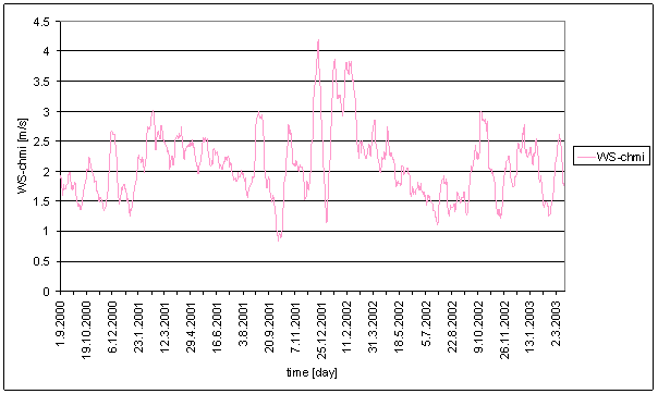
Figure 209 – Time dependence of WS-chmi irregular component

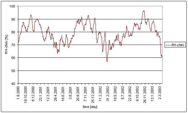
Figure 210 – Time dependence of RH-chmi irregular component

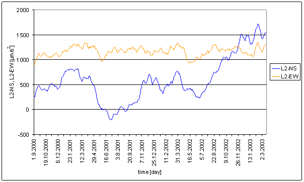
Figure 211 – Time dependence of L2-NS and L2-EW irregular component

Hypothetical transfer function f must give the same output as response to irregular input signal component or as response to periodic component or on any combination. The output depends only on input value.

If hypothetical transfer function exists, it must manifest itself as response to maximum value input signal component. The supposed behaviour must be component frequency independent and periodic or irregular component independent i.e. the same transfer function must be valid for every frequency of periodic component and the same transfer function must be valid for irregular component.

Additionally, if one input signal type (periodic or irregular component) is considerably greater than the second one, the same difference must be in output signal. Therefore only signals with the same or similar periodic to irregular component ratios can have causal relationship.

If the ratio is considerably different, it is impossible that output signal can be generated from input signal by any type of nonlinear transfer function f with constant parameters.

Transfer function f must be valid and must be the same function in whole compared time period to enable hypothesis success i.e. the signals have causal relationship. It means, that transfer function f must be the same in any time and must give the same output for the same input (with respect of possible errors).

It is the reason, why irregular to periodic component ratio of all signals was analyzed in first step. In second step irregular component time correspondence was analyzed, especially the signals with irregular component considerable greater than periodic one.

Limits were specified as follows:

L₁= 10*Amax

L₂= 5*Amax

Where:

L₁is signal value maximum and minimum difference in whole analyzed time period

L₂ is sliding average maximum and minimum difference in whole analyzed time period. Amax is spectral line maximum amplitude computed by STFT in 96day window.

The criterion differentiates signals with high irregular component (irregular part 2.5times greater than maximum periodic component) from other signals.

Irregular and periodic component ratios analysis results are in following table.

Table 32 – Periodic and irregular signal components ratios

Signal component ratios comparison gives following signal groups:

A Group with dominant irregular component and very low periodic component. Amax is maximally 3% of irregular signal range. The A group contains T-int, P-chmi, TD-chmi, L2-NS and intRA-uexp t=600hour.

B Group with great irregular component and low periodic component. Amax is maximally 20% of irregular signal range. The B group contains L2-EW, T-ext, T-chmi and intRA-uexp t=120hour.

C Group with comparable irregular and periodic components. The ratios are close to L₁and L₂ limits. The C group contains WS-chmi and RH-chmi.

D Group with low irregular component and high periodic component. The ratios are below L₁and L₂ limits. The D group contains RA-chmi, RA-uexp, SS, SSS and intRA-uexp t=24hour

Measured displacements are members of A and B groups. It has no sense to analyze dependency of measured displacements on signals from other groups (C and D). Only signals from C group could be analyzed for sure.

The strong dependency of intRA-uexp on t parameter value is interesting. t=120hour enables correspondence of intRA-uexp with L2-EW. t>600hour enables correspondence intRA-uexp with L2-NS.

Relation between synchronously measured displacements (L2-NS, L2-EW) and external effects sliding averages are shown on following figures. One graph point is determined by averages computed from the same time interval of both compared signals. If hypothetical transfer function f exists, it must be seen in the graph.

Following figures show relations between signals from A and B groups. Other group signals are shown only for completeness.

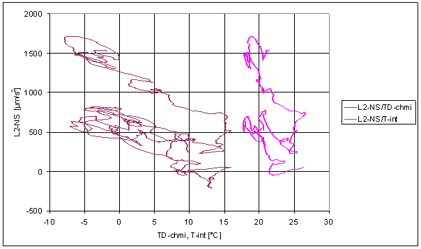
Figure 212 – Sliding averages dependence of L2-NS on TD-chmi and T-int

Figure 213 – Sliding averages dependence of L2-NS on P-chmi

Figure 214 – Sliding averages dependence of L2-NS on T-chmi and T-ext

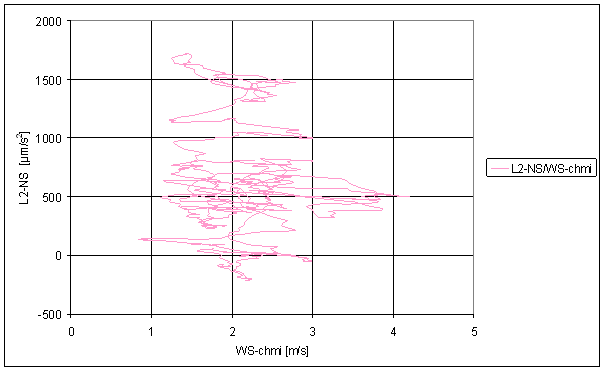
Figure 215 – Sliding averages dependence of L2-NS on WS-chmi

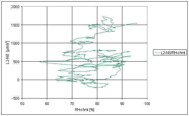
Figure 216 – Sliding averages dependence of L2-NS on RH-chmi

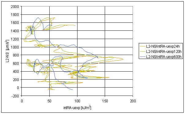
Figure 217 – Sliding averages dependence of L2-NS on intRA-uexp t=24hour, intRA-uexp t=120hour and intRA-uexp t=600hour

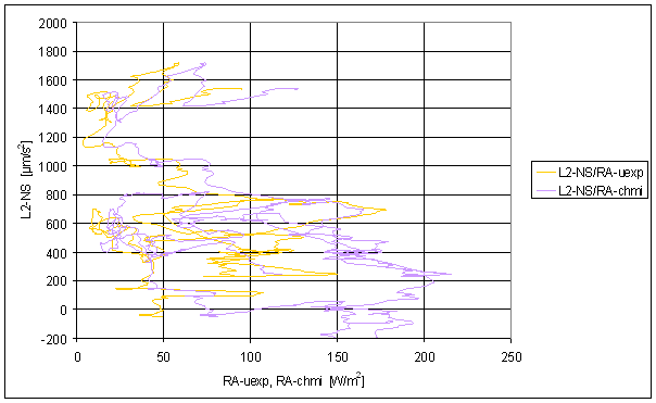
Figure 218 – Sliding averages dependence of L2-NS on RA-chmi and RA-uexp

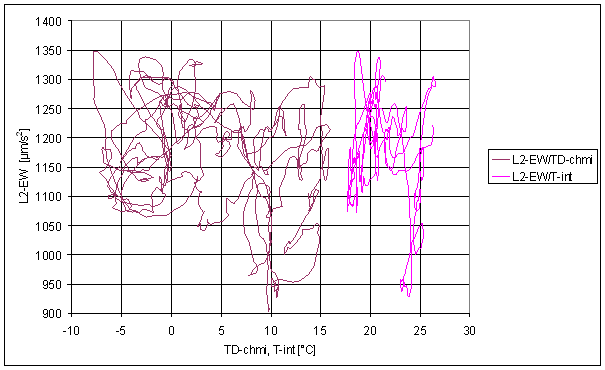
Figure 219 – Sliding averages dependence of L2-EW on TD-chmi and T-int

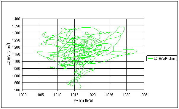
Figure 220 – Sliding averages dependence of L2-EW on P-chmi

Figure 221 – Sliding averages dependence of L2-EW on T-chmi and T-ext

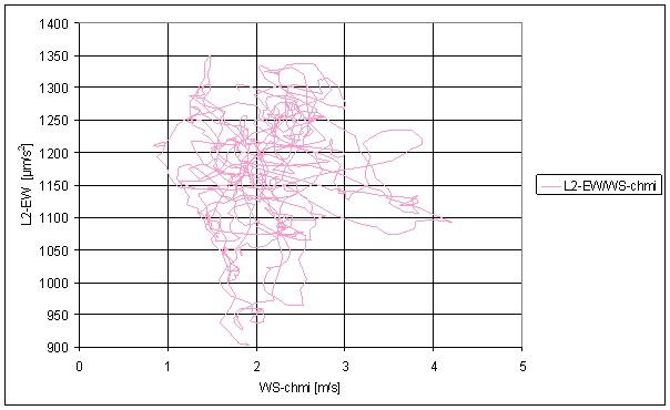
Figure 222 – Sliding averages dependence of L2-EW on WS-chmi

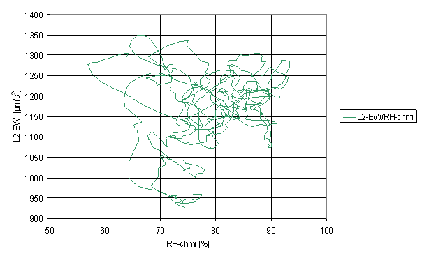
Figure 223 – Sliding averages dependence of L2-EW on RH-chmi

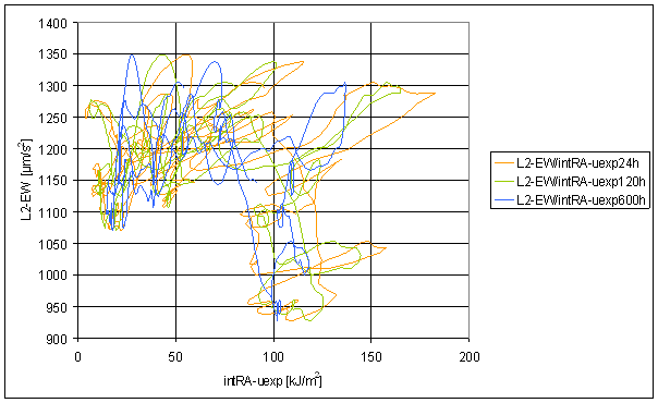
Figure 224 – Sliding averages dependence of L2-EW on intRA-uexp t=24hour, intRA-uexp t=120hour and intRA-uexp t=600hour

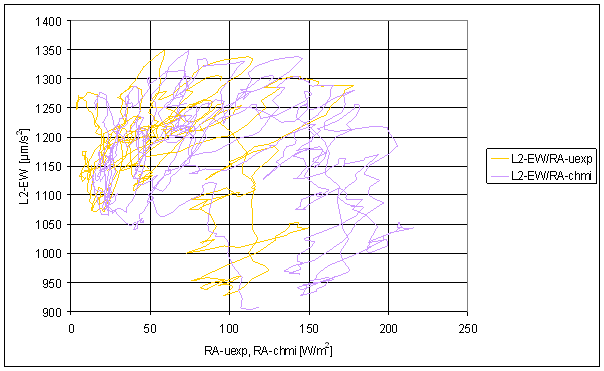
Figure 225 – Sliding averages dependence of L2-EW on RA-chmi and RA-uexp

The displayed sliding averages dependences show no possibility to approximate transfer function between any external signal from any group and measured displacements by time independent nonlinear transfer function f.

Transfer characteristics of L2-NS /TD-chmi, L2-NS/T-int, L2-NS/T-chmi and L2-NS/T-ext enable considering approximation by set of parallel straight lines. It means linear function f with step time dependent L2-NS offset. These offset steps can not be physically eliminated. Long-term measuring device stability was not proved this way, to enable eliminating of random starting value errors. The errors can cause offset change in steps.

This hypothetical approximation means that L2-NS irregular component is linearly dependent on irregular temperature component in range of annual temperature changes.

In this case any measured L2-NS value must be linearly dependent on any temperature value. It must be valid for irregular and periodic components. It is in conflict at least with spectral analysis results.

The L2-EW measured displacements component (it has good spectrum correspondence with intRA-uexp) nonlinear hypothetical function analysis gives this result: there is no transfer function enabling use of linear or nonlinear transfer function f with constant parameters for irregular component approximation. It is very important result because irregular component of L2-EW and considered external effects signals (including intRA-uexp) are many times greater than periodic component.

Comparison

No visible transfer function f was displayed in previous section. This section shows results of analysis computed by the same method as in previous section applied on signals with known relation for comparison.

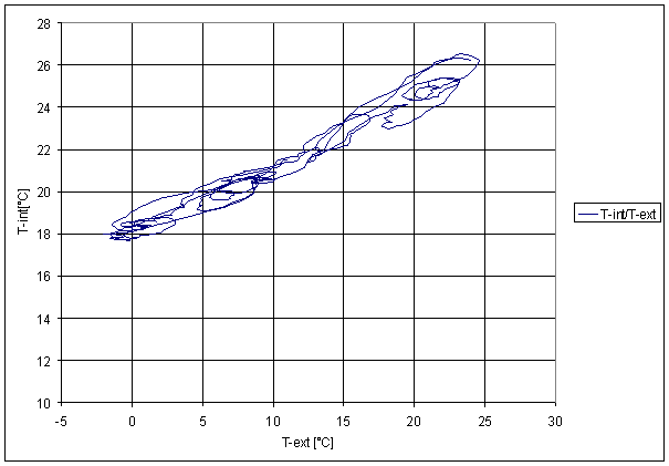
Figure 226 – Sliding averages dependence of T-int on T-ext

Figure 227 – Sliding averages dependence of T-ext on T-chmi

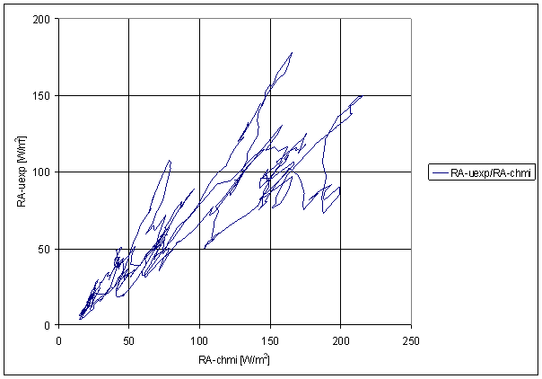
Figure 228 – Sliding averages dependence of RA-uexp on RA-chmi

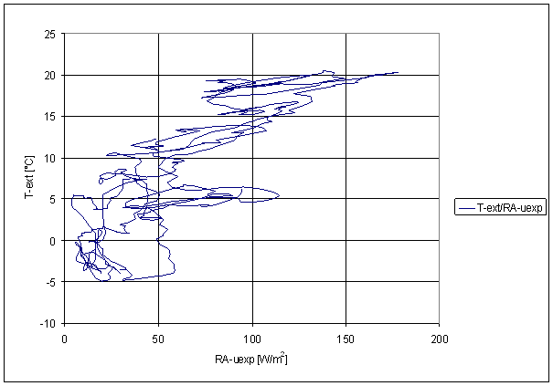
Figure 229 – Sliding averages dependence of T-ext on RA-uexp

Figure 230 – Sliding averages dependence of T-ext on intRA-uexp

The results show very visibly the possibility to approximate transfer function f and character of the function. It works in cases if there is no direct local causality between physical quantities (e.g. RA-chmi and RA-uexp) or if there is only partial causality (e.g. external temperature and Sun radiation). In all these cases linear or nonlinear character and basic shape of the transfer function f is visible.

Summary

Sliding average analysis of irregular signal components shows that no nonlinear relation between measured displacements and external effects exists. Only L2-NS component enables considering approximation of transfer function f by linear transfer function of temperature (TD-chmi, T-int, T-chmi and T-ext).

The L2-EW measured displacements component does not enable any transfer function approximation by any type of time invariant transfer function f.

These results are in contrast with spectrum analysis result. Analysis of greater component (irregular) gives other results than spectrum analysis of smaller component.

It is not possible that two different transfer functions exist for one system in the same time, one for irregular component and another for periodic component. It is possible to formulate global conclusion.

None of measured displacements component (L2-NS and L2-EW) has good correspondence for irregular and periodic component with any analyzed external effects signals.

Nonlinear dynamic system

It is not possible generally analyzed general nonlinear dynamic system behaviour, especially dynamic system with time dependent parameters by comparing input and output signals.

The nonlinear dynamic systems have behaviour similar or to linear dynamic systems or to nonlinear static systems in case, if the nonlinearity is small in comparison with signal amplitudes or in case, if system time constants are out of analyzed frequency spectrum. This system types were analyzed in previous sections.

The situation is considerably different in case if nonlinearity is dominant and dynamic parameters dominantly drive system behaviour in analyzed spectral range. This system can have generally any behaviour. It can generate its own oscillations or chaos signal [20].

Let us analyze local impacts on measurement system in our case. Measurement system has very small relative deflection (maximally 10^-4 of its physical range). The absolute deflection is very small too (maximally 0.1 mm). Analysed spectral range is about 1hour to 2500 hours. Existence of this nonlinear local effect is physically almost impossible. More precisely, it is not known any physical effect with dominant nonlinear behaviour in these small deflections and with time constant in range from hours to several days. Only both conditions together are essential conditions for nonlinear dynamic system behaviour.

The displacements were measured in many different localities (10 different localities). In all localities were measured significant displacements and clear periodic displacement were measured in majority of localities. The hypothetical local nonlinear dynamic system would have to exist in all these localities and therefore the system would have to be independent on different construction and different materials used in the buildings where the measurement device was located.

Parameter time dependence was studied too. Space and material configuration surrounding the measurement device and measurement device are time stable. Only material ageing exists. It is slow irregular effect. The fact enables to eliminate dominant impacts of changing parameters of surrounding terrain, buildings and measurement device and therefore time transfer function parameter time dependency generated by local impacts.

The local effect must be clearly separated from global parameter time dependence effect. The Sun-Earth system has clear time dependency with respect of earth surface. And the Sun-Earth system has great influence on many different quantities on the earth surface. These quantities contain the Sun-Earth system time dependency in their signals. The only cause is the Sun-Earth system. It must not be supposed that one quantity is cause of another one based only on the same or similar time dependency. It is not possible to made conclusion like air pressure is dependent on relative humidity because both signals contains similar periodic signal spectral lines. The only right conclusion should be that the signals have common partial cause and it is the Sun–Earth system. Conclusion about dependency of one quantity on another must be based on other facts.

The same conclusion can be made for L2-NS and L2-EW measured displacements (and for measured displacements in other localities).

Measured displacements have at least partial cause in the Sun–Earth system.

Anthropogenic impacts

Anthropogenic impacts (human activities) are another working hypothesis. Different shakes, mass transfer, electric power system and other electromagnetic man-made noise, etc. can have dominant influence on measured displacements.

Only mass transfer can be theoretically eliminated. Other impacts must be analyzed.

Effect comparable with measured displacements can be caused by transfer of 200m diameter sphere made from earth mass average density material. The mass transfer would have to be made regularly with 24 hour period in immediate neighbourhood of measured device. It would have to be made in all localities where clear periodic component was measured. This great mass periodical transfer does not exist.

Anthropogenic impacts have 24hour period. The 24 hour rhythm is the most frequent anthropogenic cycle. Anthropogenic impacts have other own time patterns.

Measured fluent curves with no quick value changes are not typical for anthropogenic impacts.

Typical anthropogenic time characteristics are week dependency and summer time changes.

Practically all human activity in Czech Republic (only human activity in this area can have local influence to measured displacements) have week cycle with rare national holiday and two one hour shifts during the year.

This time characteristics were not recognized from measured displacement analysis.

One week period (168 hour) must be visible in global 2 year spectrum if exists. See following figure.

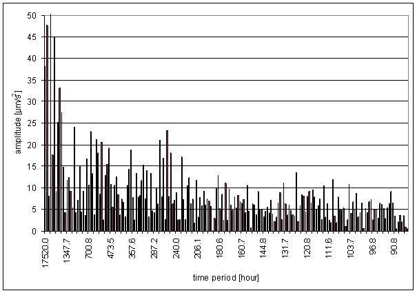
Figure 231 – Slow processes spectrum part – L2-EW

Period close to 10.6 day (254 hour) is the greatest spectral line in the analyzed area. The period can not be caused in artificial human activity.

Time shift connected with daylight-saving time begin and end should result into decomposition of 24 hour, 12hour and 8hour spectral lines in global spectrum. This decomposition should be the same as is in spectral analysis result (described in previous sections). The decomposition can not be differentiated from the same effect caused by spectral line time dependency with 1 year period. The time shift does not cause time dependency of spectral line. Conclusion is: global spectrum can not be used for analyzing time shift existence.

STFT analysis is very sensitive for periodic signal shift in time. This time shift moment must be visible in STFT result.

It is possible to use STFT. Asymmetry in subdominant frequency lines displays clearly time shift. This frequency line asymmetry clearly signals “slowing down” and “acceleration” of periodic process in the right time change interval. The difference of spectral lines symmetrical to basic spectral line shows the time shift best way. Following figure shows simulated summer time change (28^th March and 27^th October) results.

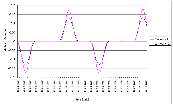
Figure 232 – Simulated summer time change displayed by relative frequency shift in simulated 24 hour periodic signal with random amplitude

The same analysis of measured displacements is on following figure.

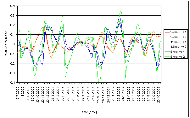
Figure 233 – Relative frequency shift in measured displacements signal L2-EW

Measured displacements spectrum asymmetries are 3 times or 4 times a year (7 times in 2 years). The summer time changes are only 2 times a year. The summer time changes are in fixed times close to 20^th March and 20^th October every year. Autumn frequency change is positive and spring frequency change is negative.

Conclusion is: measured displacements spectrum asymmetry is not caused by timing connected with human activities in the area of measurement.

Let us compare basic anthropogenic impacts influence in different measurement localities:

L1 and L10 are placed in small village located out of the main traffic (roads, railways, airlines). No exploitation is in neighbourhood. Only standard agriculture activities and recreation activities are in neighbourhood.
L2, L7 and L9 are placed in Prague suburb about 100m far from underground line and about 200m from medium loaded road. Only low local traffic and no transit traffic are close to the localities. The localities are close to airline corridor near airport Prague-Ruzyně. No railway is near the localities.
L3 is placed in Prague suburb. No railway or underground line is near the locality. Road with transit load is placed about 300m far from the locality. No airline corridor is close to the locality.
L4 is placed close to the high loaded railway in centre of Prague. Medium traffic road including tramway traffic is located about 100m far from the locality. No airline corridor is close to the locality.
L5 is placed in village close to Prague. It is placed about 200m far from heavy loaded highway. No railway, underground or airline corridor is close to the locality
L6 is placed in Prague suburb. No transit traffic is close to the locality. Only very low local traffic exists close to the locality. Airline corridor to Prague-Ruzyně airport is close to the locality. No railway or underground is close to the locality.
L8 is placed in Prague suburb. No transit traffic is close to the locality. Only very low local traffic exists close to the locality. Airline corridor to Prague-Ruzyně airport is about 2km from the locality. No railway or underground is close to the locality.

The localities have highly different anthropogenic impacts conditions. Measured displacements are not correlated with different human activities in different localities. Measured displacements must be caused by other effect than human activities can be deduced from the previous analysis.

Other important argument is great correspondence of L2-EW measured displacement component global spectrum and spectrum time dependency with RA-uexp and with SSS signals ones. Both signals are physically based signals independent on human activity.

Subsoil tilt

Subsoil tilt can cause measurement weight deflection like direction change of gravity gradient. These two possible causes of weight deflection can not be differentiated from one measurement. Measurement principle is based on gravity gradient measurement relatively to the measurement device surrounding.

Results measured in two very close localities measured in the same time can be compared. They can be used for subsoil tilt elimination. They can not be used as proof of subsoil tilt influence.

It is valid especially if the two measurement localities are above the same subsoil. The L2 and L7 localities are in the same place. The only difference is in altitude. L1 and L10 locality are very close each other. The difference is in altitude and in small locality shift.

Simultaneously measured results in these localities shows that measured displacements can not be caused only by subsoil tilt or building tilt.

The measured displacement would have to be the same or very close to each other and exactly synchronous in case of any surrounding tilt. The surrounding tilt and measured tilt must be the same if gravity gradient is unchanged. It must be valid in both axes components and in any time.

Important correlation exists between simultaneously measured displacements in L2 and L7 localities. It is not agreement corresponding with the same tilt in these localities. It is valid by analogy in L1 and L10 simultaneously measurements.

Figure 234 – Simultaneously measured trajectory in L2 and L7 localities

Figure 235 – Time dependency of simultaneously measured displacements in L2 and L7 localities

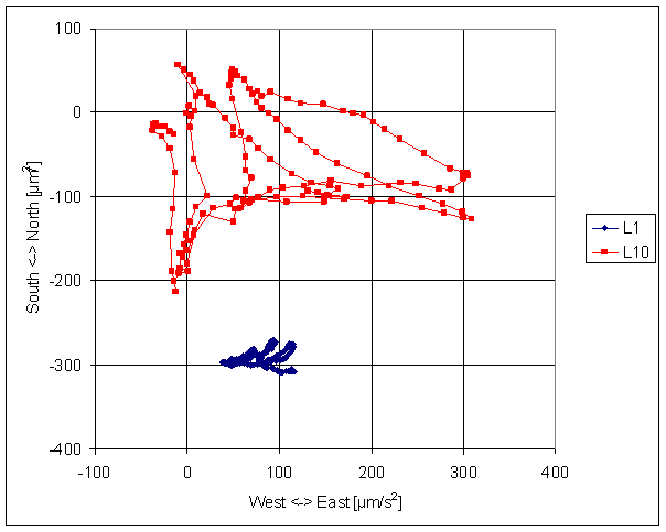
Figure 236 – Simultaneously measured trajectory in L1 and L10 localities

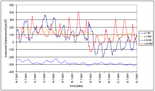
Figure 237 – Time dependency of simultaneously measured displacements in L1 and L10 localities

Wind impact

Wind can not be the cause of measured displacements in L2 locality. It is result of periodical and irregular component comparison in previous sections. L2 locality is placed about 20m above the terrain in tall building. Wind impact to tall buildings is well-known effect. Measuring device is in principal very sensitive to building movement.

This section deals with wind impact value on measured displacements in L2 locality.

The time period with maximum wind speed was selected from total measured time range. Wind speed WS-chmi was used for the analysis. Analysis results are in following figures.

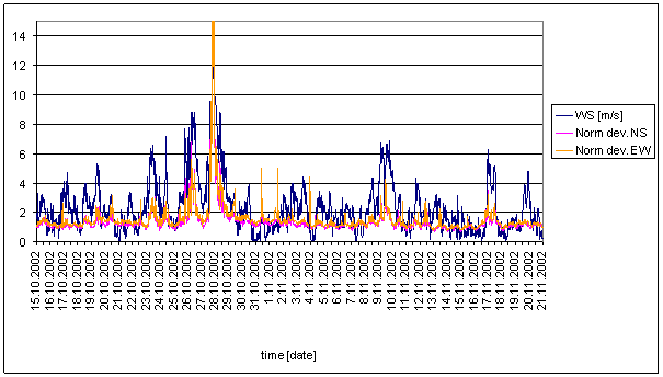
Figure 238 – Deviation comparison of wind speed WS-chmi and standardized measured displacements L2-NS and L2-EW. Measured displacements deviations were standardized by one constant coefficient to enable displaying in one common graph with wind speed in [m/s]. Measured displacements deviations have no physical units in the figure.

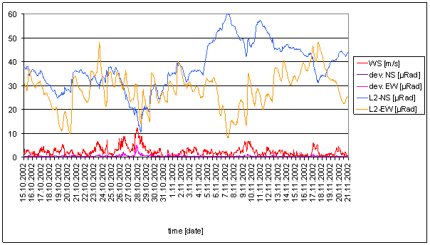
Figure 239 – Comparison of wind speed WS-chmi, L2-NS and L2-EW measured displacements values and deviation. All measured displacements in this graph are standardized by the same constant to enable relationship display. Measured displacements unit micro radian was selected.

Measured displacements deviations are in correlation with the wind speed especially with the highest wind speed are in good correlation with some local maximum of measured displacements deviation.

Maximum wind speed has impact to measured displacements deviation. The wind speed is not the only impact on measured displacements deviation. Wind has low or no impact if the wind speed is medium or low. It is great majority of the time.

Average measured displacements are not affected by wind speed. The maximum measured wind speed about 12m/s has made no dominant change in averaged measured results.

Building deformation impact

Measured deflection can be caused by building deformation. The measurement device was fixed to the building wall and ceiling. Any horizontal relative movement of the weight hanger or the microcamera holder can be interpreted as measured displacements and misinterpreted as a gravity gradient change.

Buildings are strained by many external effects. The external effects were analyzed in previous sections. The building deformation can be one special hypothetical system from generally analyzed ones in previous sections. The general analysis did not find any local system with dominant impact to measured displacements.

Even so let us analyze building deformation impact separately.

The working hypothesis is: Measured displacements are caused only or dominantly by building deformations. The building deformations are caused by known physical external effects especially external temperature or Sun radiation or combination.

This hypothesis looks very probable with respect of 24hour periodical part amplitude correlation results.

Following table shows 24hour periodic component amplitude correlations of measured displacements and T-ext, RA-uexp, intRA-uexp. The correlations were computed from measured values in time period from September 2001 to July 2003.

Table 33 – 24hour amplitude correlation of external effects and measured displacements in L2 locality

Following figures show correlation graphically.

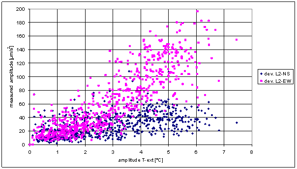
Figure 240 – 24hour amplitude correlation of external temperature T-ext and measured displacements in L2 locality

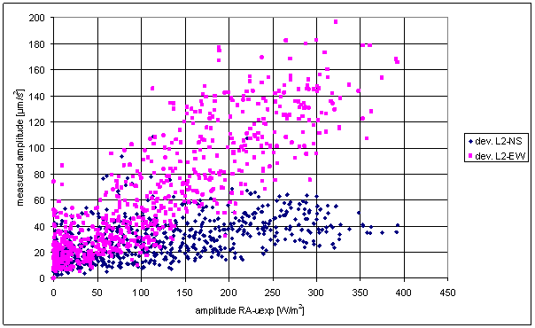
Figure 241 –24hour amplitude correlation of Sun radiation RA-uexp and measured displacements in L2 locality

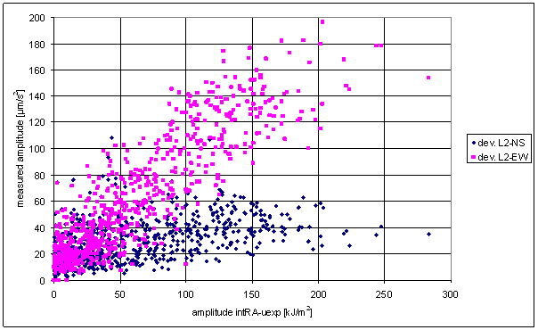
Figure 242 – 24hour amplitude correlation of integrated Sun radiation intRA-uexp and measured displacements in L2 locality

Let us study possible causality between measured displacements and external temperature or Sun radiation in measuring locality.

Microcamera holder was fixed to the wall. The wall is flat physical element. One dimension is considerably smaller than other two dimensions. The wall thickness is several times smaller than wall width or height.

Let us analyze measured displacements orientation against the wall. If the wall deformation caused some dominant deflection, the measured results would have to be different in direction parallel with the wall and in direction orthogonal to the wall.

Following figure shows measurement results from different localities (all localities where great 24 hour period signals were measured) oriented relatively to the wall holding microcamera. The results are in raw coordinates X, Y. The raw coordinates are microcamera body relative coordinates and they are fixed the same way relatively to the wall in every locality.

Figure 243 – Raw measured displacements trajectories in different localities oriented to the base wall

Microcamera optical field X axis is parallel with the wall and Y axis is orthogonal to the wall. Results are displayed without any filtration or other processing. Only offsets were used to enable display all trajectories in one figure. No pendulum rod length correction was applied.

The figure shows raw measured displacements signal/noise ratio.

Measured trajectories do not contain any extraordinary direction, especially any direction correlated with wall orientation.

Conclusion is: The wall deformation can not be the dominant cause of measured displacements.

The measured deflection can be caused by wall to ceiling relative movement.

The weight hanging wire (pendulum rod) was fixed to the wall in L8 and L10 locality instead of the ceiling. It was not technologically possible to fix the wire to the ceiling in these localities. The measured deflections in L8 and L10 localities can not be caused by ceiling to the wall relative movement.

Conclusion is: The wall or ceiling movements was not recognized in measured displacements.

Whole building can move. Whole building can be reformatted by external effects. Temperature dependence of different construction materials and non-uniform heating must cause some maybe very complicated building deformations of unknown size. This movement can have influence to the measured displacements.

Following figure shows L2, L7 and L9 locality building scheme with relative locality position.

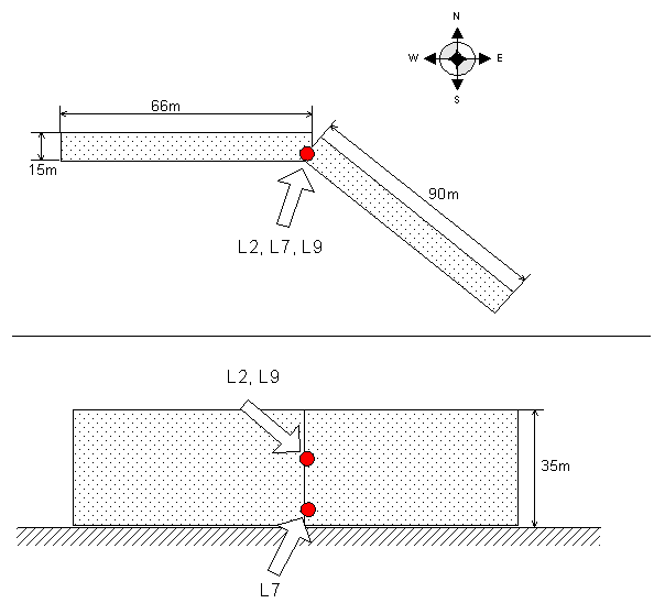
Figure 244 – L2, L7 and L9 locality position schema

The building is very long, cranked and very high. Measurement localities are close to break point. Dominant building direction is East-West. The building is many times longer in east-west direction than in north-south direction.

South site of the building is heated by Sun radiation many times more than other sites. These factors support greater building deformation in north-south direction than in east-west one.

Measured displacements results show considerably better external temperature and Sun radiation correlation with measured displacements east-west component (L2-EW) than with north-south one (L2-NS).

East-west measured displacement component amplitude is about two-times greater than north-south one but the building is more than 10times longer in east-west direction than in north-south direction.

Measured displacements are vectors. A vector draws trajectory during time. Measured trajectory is not section of a line. It is frequently closed curve similar to ellipse.

The cause can not be scalar. The cause can be two independent scalars with orthogonal impact or vector.

Temperature is scalar with no direction. The directional impact of temperature can be caused only by body shape change influenced by temperature. Closed curve can be caused by temperature only in very special circumstances.

The circumstances are:

Direction dependent hysteresis – other behaviour in case of temperature increasing and other behaviour in case of temperature decreasing with different values of the effect in two orthogonal directions.
Direction dependent phase delay – phase delay comparable with main period (24 hour) different in two orthogonal directions.

It means that all buildings with very different shapes and very different materials would have to have the special body shapes and materials with special material features.

It is unknown feature of bricks or concrete or other building material to have temperature extensibility hysteresis dependent on direction. The bricks are randomly oriented in the wall. No correlation between wall orientation and measured displacements was found in previous analysis. The measured deflections are very small (less than 0.1mm).

Phase delay difference in two axes must be comparable with 24 hour period. The phase difference must be in hours to enable closed curve trajectory. Measurement results show very quick reaction of measured displacements on external conditions change (in minutes) in both directions. It is not compatible with “needed” phase delay difference (in hours). These results were measured in case of quick whether changes and they are described in following description in this section.

Frequency spectrum comparison and irregular part comparison of external temperature and Sun radiation with measured displacements were described in previous sections together with other external effects. The building deformation can be special case of general systems analyzed in these sections.

The results are:

L2-NS spectrum is very different from all other external effects signal spectrums.
L2-NS irregular component time dependency can be correlated per parts with external temperature irregular part by linear dependence
L2-EW spectrum has the best correspondence with intRA-uexp signal (integration of local Sun radiation)
L2-EW irregular component time dependency can not be caused by any external effect irregular component

Periodic and irregular parts dependencies are not equal. L2-EW component shows possible correspondence with other external effect and in other time period range (periodic component or irregular component) than L2-NS one. Possible linear dependency of L2-NS irregular part is not validated by periodic part spectrum comparison. Spectrum similarity of L2-EW with local Sun radiation was not validated by irregular component analysis.

We can study season dependency as well.

If external temperature was the dominant cause of measured displacements, similar temperature difference would have to cause similar measured displacements. Following figure displays relations between measured displacements and external temperature in two different seasons.

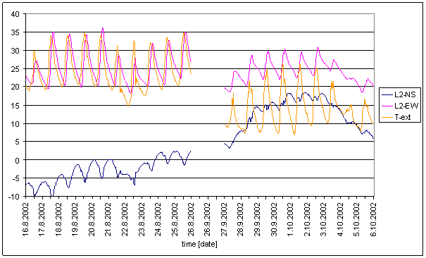
Figure 245 – Comparison of external temperature T-ext and standardized measured displacements amplitudes in two time periods in L2 locality. The graph was made this way, that offsets and amplitude coefficients was chosen to give the best correspondence between L2-EW and T-ext in first season. The same transformation was used for second season.

The graph shows that in the second season the hypothetical correspondence looks quite different than in first season. The second season begins only about one month after the first season finish.

L2-EW measured displacements have about two-times lower amplitude in second season than in first one. Opposite situation is in case of external temperature. T-ext amplitude in the second season is greater than in the first season.

It could be possible only if the building temperature deformation parameters were changed more than two-times in one month.

Let us compare time dependency.

The first step is comparison of short time dependency.

Rapid external conditions changes were used for the analysis. Quick weather change brings this rapid change of external conditions.

The days with quick weather change was selected from measured time series. Following figures show measurement results from days with very quick isolated weather change.

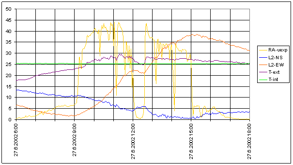
Figure 246 – Measured quantities from 27.6.2002 in L2 locality

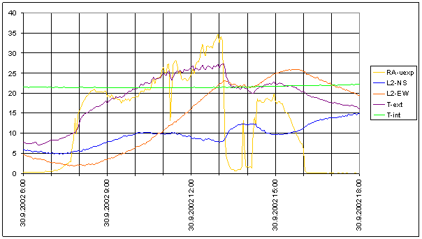
Figure 247 – Measured quantities from 30.9.2002 in L2 locality

The results from days with sharp change of Sun radiation and external temperature show that L2-NS and L2-EW measured displacements change their shapes in the same time as Sun radiation and external temperature i.e. in the time of weather change. The measured displacement changes are different from any external effects changes.

Recognized and interesting features should be:

The measured displacements change its derivation and Sun radiation changes its value.
The measured displacement change occurs when Sun radiation stops or starts.
L2-EW measured displacements values were greater in the afternoons than in the mornings in all cases.
T-ext values were not greater in the afternoon like other days with cloudless weather.
The Sun radiation RA-uexp was not greater in afternoon than in the morning.

Immediate and strong reaction of measured displacements to weather change (at most several minutes) is in contradiction with measured temperature time constant of the building. The time constant was analyzed from frequency dependence of internal to external temperature ratio. The building time constant is at least 300 hours. The value agrees with fact, that the building is constructed and used as residential house with good temperature insulation.

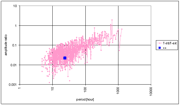
Figure 248 – T-int / T-ext frequency characteristic

Measuring device was placed inside the building in temperature insulated room. The building deformation can be caused only by temperature change of great amount of building mass. Great amount of building mass is temperature insulated. The building mass temperature change needs many hours and it is impossible in minutes.

Very short reaction time of measured displacements is in conflict with long time needed to change building mass temperature.

The second step is comparison of long time dependency.

Following figure shows different seasons measured trajectory comparison.

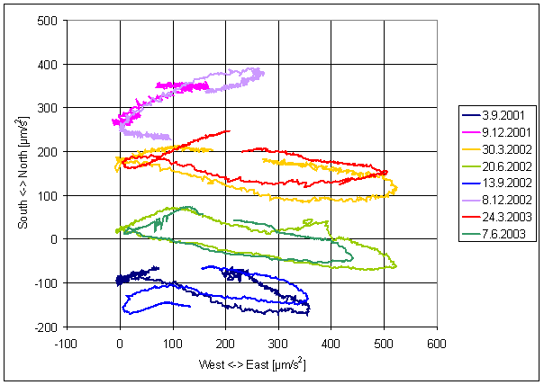
Figure 249 – Measured long term trajectory dependency in L2 locality

The Sun effects geometry on the Earth surface is equivalent in spring and autumn seasons, especially in spring and autumn equinox. The geometry differs in winter and summer solstice. The trajectory shapes and sizes repeat in 1 year period.

Measured displacements have different season behaviour. Spring equinox trajectory is very similar to summer solstice trajectory. Spring and autumn equinox trajectory are very different.

Measured trajectories change their attributes, not only the size.

It means:

Excitation quantity must change its space characteristics during the year.
The excitation quantity can not be scalar. It must be a vector.
Changes are repeatable with 1 year period. The cause must be repeatable with the same period.

There is possibility of non-uniform building heating by the Sun; it means vector interaction between the buildings and the Sun. The interaction vector has clear time-space behaviour. It is done by the Sun–Earth system time dependent geometry. The system has 24 hour basic period and 1 year period. The Sun–Earth system rotation direction in horizontal plane on the Earth surface is only one and constant in any place in the measurement area (small part of north hemisphere).

Some measured trajectories in previous figure have parts with opposite rotation direction than other part one in one day. The measured trajectories change their rotation direction in one day.

Following figure displays rotation directions in different localities. The figure shows trajectory from one selected day only (0:00 – 23:30) in 30 minute steps from one location. This full trajectory is named Lx. The partial trajectory from the same day (6:00 – 12:00) is displayed by other colour and named Lx-. This time asymmetry shows rotation direction and phase with respect of the Sun relative position.

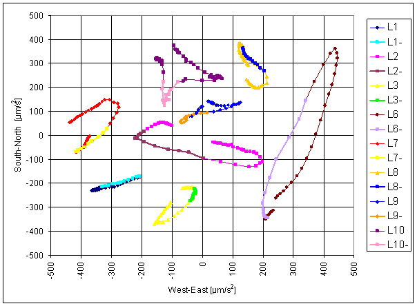
Figure 250 – Measured displacements trajectories in different localities with displayed orientation

The results are:

Measured trajectories in some localities have the same rotation direction as direction of virtual Sun movement on the sky (L3 and L6)
Measured trajectories in some localities have opposite rotation direction as direction of virtual Sun movement on the sky (L2, L7, L8, and L10)

Conclusion is: The Sun radiation can not be the cause of measured displacements minimally in localities where the rotation direction is opposite to the Sun one.

Spectrum time dependency of measured displacements and external effects connected with building deformations is analyzed in this part. Following figure shows 24hour spectral line relative amplitude time dependency.

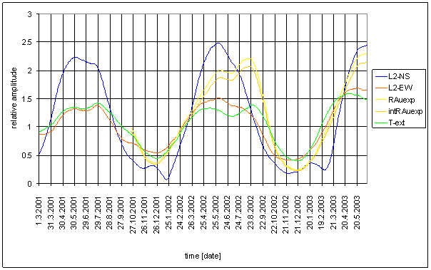
Figure 251 – Relative 24 hour amplitude time dependence in L2 locality. The Sun radiation measurement in L2 locality was made from autumn 2001. Any spectral line amplitude was standardized to their own average amplitude.

Great differences between maximum and minimum values of standardized quantities are result of the analysis. If any causality exists between quantities, standardized spectrum time dependence must be very similar as in maximum/minimum ratios, as in time shape dependency.

The greatest relative value from all quantities has L2-NS. The lowest relative value has L2-NS as well. No other quantity has comparable values.

L2-EW is close to the T-ext. It is not the same shape, but similar. Other frequency spectral lines time dependency of L2-EW and T-ext are quite different (see analysis results in previous sections). Sun radiation relative spectrum time dependency is about in the middle between L2-NS and L2-EW, but the shape is not equal.

We can compare time relations between quantities. We can see time difference between measured displacements and external effects near autumn equinox. The RA-uexp, intRA-uexp and T-ext are delayed about 30 days after L2-NS and L2-EW (they have the same relative value about 30 days later). Another situation is in winter. L2-NS is delayed about 1 month after RA-uexp, intRA-uexp and T-ext. It is not possible, that the building “saves” about 30 periods. It is not possible, that cause is delayed after result.

Let us compare in detail situations in spring and autumn equinox season. The physical situation in spring equinox is very similar to the situation in autumn equinox. The Sun–Earth system geometry is equal (only small differences in the Sun system configuration exist). The Sun radiation is the same. Previous winter or previous summer can have small influence to external temperature (caused by the Earth surface temperature capacity and other weather effects).

Following figure compares selected days with no or very small cloudiness close to equinox in two years.

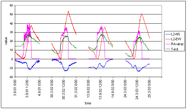
Figure 252 – Comparison of measured displacements and external effects in L2 locality in sunny days from equinoctial periods. Measured displacements L2-NS and L2-EW are shifted by individual offsets to enable good displaying in one graph. L2-NS, L2-EW and RA-uexp are standardized by constant parameter to enable display them in one graph with T-ext.

The figure confirms these external effects (T-ext, RA-uexp) are very similar in spring and autumn equinox, if day without clouds is selected.

L2-EW measured displacements amplitude (maximum to minimum difference) is more than 1.5times greater in spring equinox than in autumn equinox.

We can compare correlation of 24hour amplitudes time dependence.

The following graph was constructed this way. One year was divided into 4 seasons. Every season was symmetrical to the equinox or solstice. Season I is from 10^th February to 9^th May, season III is from 10^th August to 9^th November of corresponding year. Measured amplitudes intRA-uexp and L2-EW in one season are displayed by the same graphical symbol and the same colour.

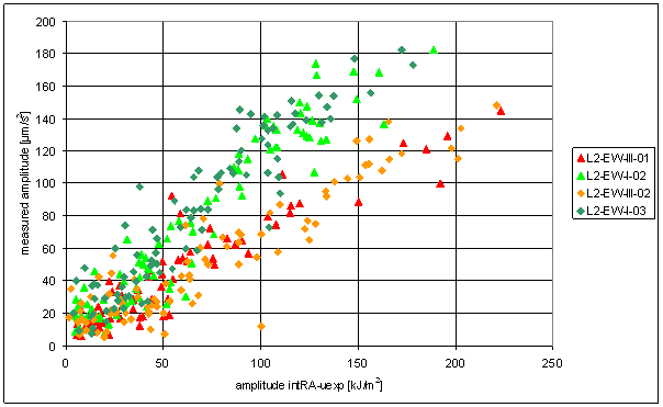
Figure 253 – 24hour amplitude correlation per season of integrated Sun radiation intRA-uexp and measured displacements in L2 locality

It is evident, that correlations in one season are better than in the whole range. It is evident, that spring equinox situation is different from autumn equinox one.

Time dependence of L2-EW 24hour amplitude to intRA-uexp one ratio is in following figure.

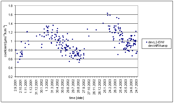
Figure 254 – Time dependence of L2-EW to intRA-uexp 24 hour amplitudes ratios in L2 locality. The graph displays only those ratios where both amplitudes are greater than average amplitude

The results are:

Amplitude ratio time dependency is periodical continuous function
Maximum to minimum ratio of the function is greater than 2
Time period is one year
Maximum is close to spring equinox, minimum close to autumn equinox
Amplitude values in winter are very frequently under average for long time (can not computed and displayed)

If L2-EW measured displacements were caused by local building deformation, physical parameters of the building should continuously change during the year the way that the deformation close to spring equinox would have to be more than two times greater than the ones close to autumn equinox. The physical parameters should be changed this way, that during season with maximum Sun radiation and maximum external temperatures must have value between values from spring equinox and autumn equinox and values similar to the parameters from winter season (with lowest Sun radiation and with lowest external temperature).

The author of the text consider this physical effect to be less probable than the measured displacements are caused by gravity gradient direction change generated by undocumented gravity interaction.

Conclusion

Main conclusion is that dominant cause of measured displacements is different from all analyzed external effects. Any analyzed external effect or any combination of external effects has no dominant impact to measured displacements.

The unknown cause has dominant impact to the measured displacements; it has its own laws. The laws are different from dependency on any analyzed external effects or their combinations.

Any external effects impact to measured displacements was not eliminated. This impact can cause measurement errors.

Those measurement errors have not value to disable study of unknown measured effect.

Following features of unknown effect were recognized:

The best correspondence of L2-EW spectrum with local radiation RA-uexp and modelled local radiation SSS (with respect of integrating transfer function). It was proved by numerically integrated signal intRA-uexp.
Different noise type of Sun radiation and measured displacements
Very good correlation between 24 hour amplitude of L2-EW with intRA-uexp with one year periodic time dependence.
Very quick and reliable reaction of measured displacements on quick weather change

The recognized features of unknown measured displacement cause enables to formulate hypothesis, that measured displacements L2-EW depend on time integral of the Sun relative movement real geometry in measurement locality. The measured displacements are impacted by building geometry close to L2 locality and by cause common with Sun radiation modification (cloudiness). It can be explained by shielding-like effects.